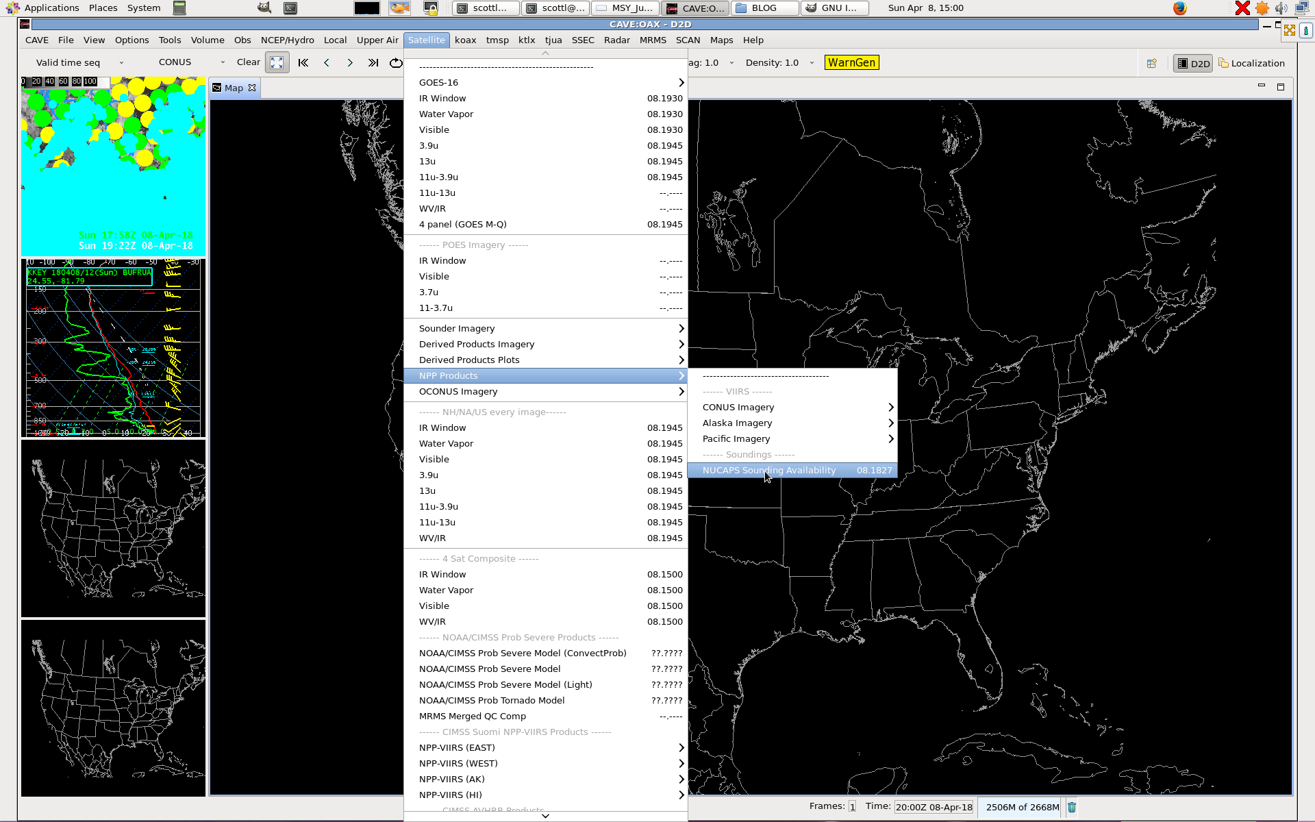
NUCAPS (NOAA-Unique Combined Atmospheric Processing System) vertical profiles have been available in AWIPS for some time now (Click here to see how to access them in AWIPS; they are also available online at this site). Legacy Atmospheric Profiles (LAP) derived from ABI Channels (and GFS Information) are available in AWIPS now as well (horizontal fields derived from LAP soundings are available online as well).... Read More
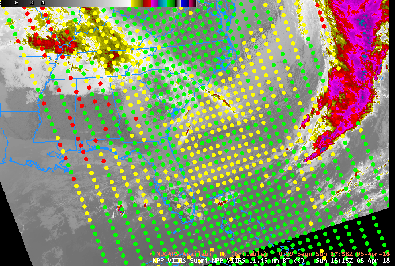
NUCAPS Sounding Availability points plotted over a VIIRS Visible (0.64 µm) image at 1815 UTC, 8 April 2018 (click to enlarge); NUCAPS Soundings from the point nearest Miami and Key West are shown below
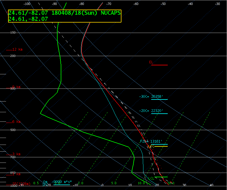
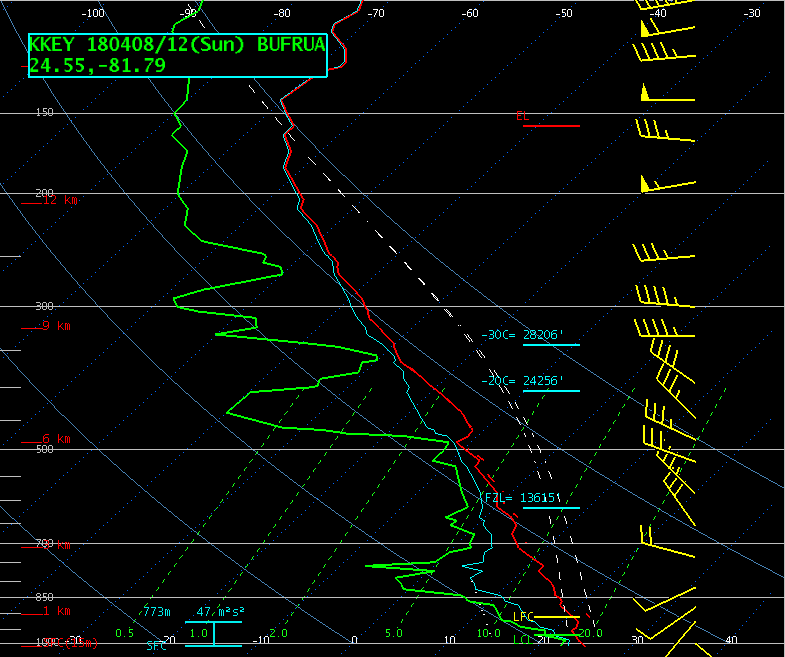
NUCAPS vertical profile near Key West FL, 18Z on 8 April 2018 (Click to enlarge)
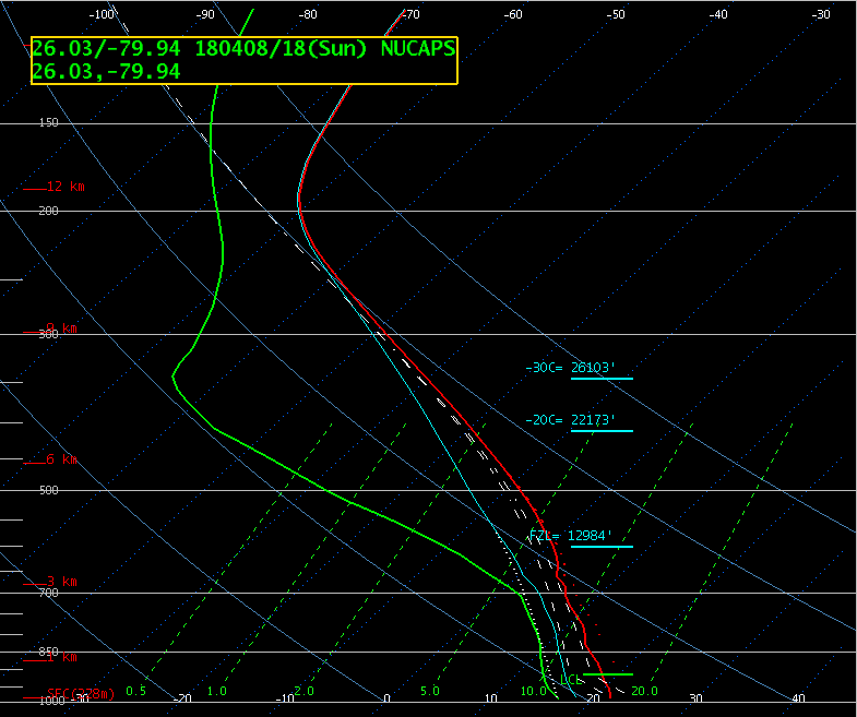
NUCAPS vertical profile near Miami FL, 18Z on 8 April 2018 (Click to enlarge)
NUCAPS (NOAA-Unique Combined Atmospheric Processing System) vertical profiles have been available in AWIPS for some time now (Click here to see how to access them in AWIPS; they are also available online at this site). Legacy Atmospheric Profiles (LAP) derived from ABI Channels (and GFS Information) are available in AWIPS now as well (horizontal fields derived from LAP soundings are available online as well). How do Legacy Atmospheric Profiles compare to NUCAPS profiles? Both are derived from satellite data. (Click here for a Quick Guide on NUCAPS; Click here for a Quick Guide on Legacy Atmospheric Profiles).
The strength of NUCAPS Soundings is that they are observation-based and independent of a model first guess (or background field). That is, they are retrieved from satellite measurements of emitted radiation at hundreds of different wavelengths in the infrared and in the microwave, with a statistical regression as first guess. In the case of NUCAPS from Suomi NPP (or NOAA-20), the data are from CrIS and from ATMS, infrared and microwave sounders, respectively. Compare the vertical profiles above to the 12 UTC soundings from Miami and Key West. There is better vertical resolution in the radiosondes, of course, but NUCAPS provides timely model-independent information at times when convective initiation might be starting.
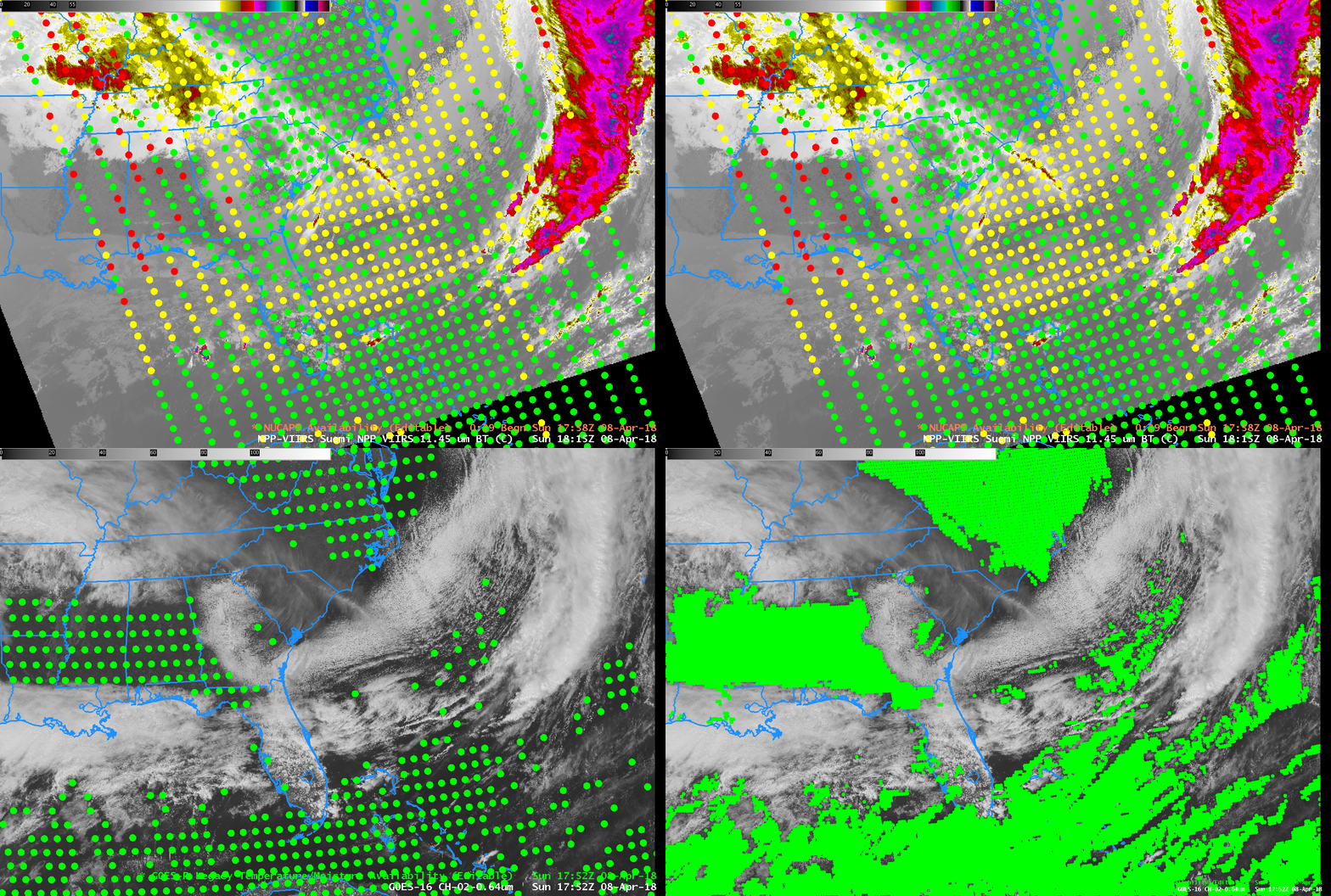
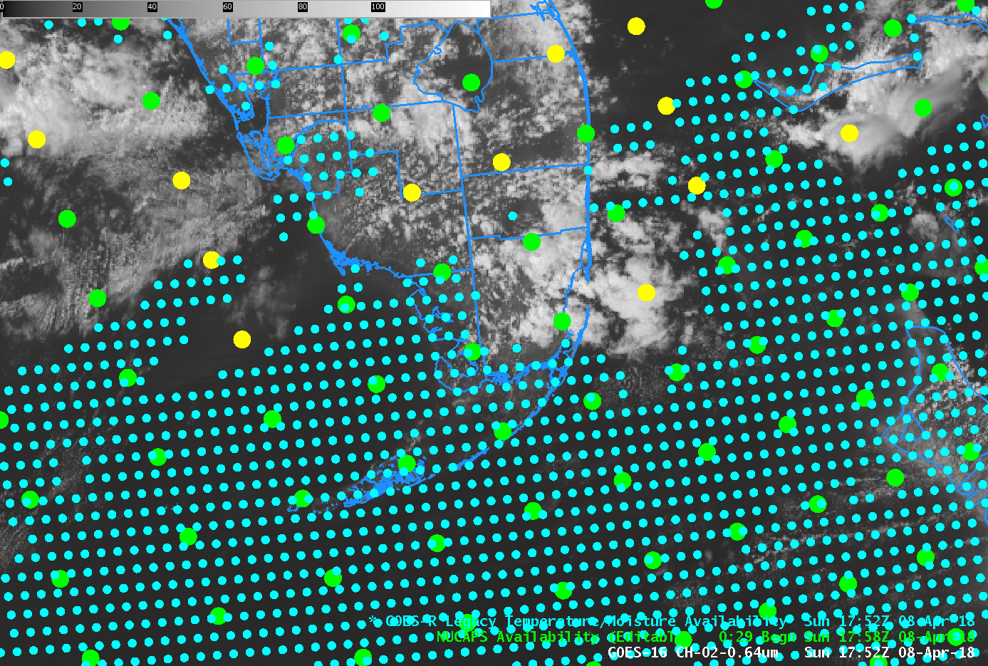
NUCAPS Soundings Availability (plotted on top of the VIIRS 11.45 µm infrared image from 1815 UTC), a subset of GOES-16 LAP Sounding Availability points (plotted on top of the GOES-16 0.64 µm Visible Image), and then all GOES-16 LAP Sounding Availability points (Click to enlarge)
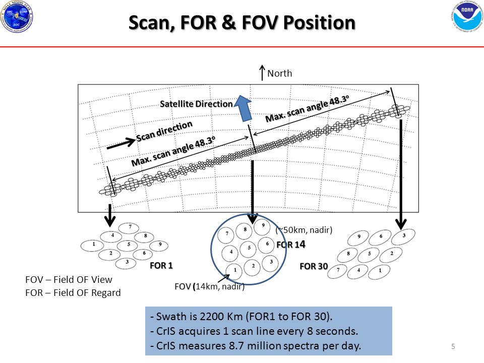
NUCAPS Soundings are produced in clear and partly cloudy conditions. This owes to the 3×3 CrIS field of regard that is incorporated into each NUCAPS profile, and to the ability of microwave imagery to produce a sounding in cloudy (but not precipitating) regions.
In contrast, LAP temperature and moisture profiles are produced only where the GOES-16 Clear Sky Mask identifies clear skies. LAP output is on a 10-km grid, however, so there are many possible soundings. The image below, zoomed in over southern Florida, shows in cyan the availability of LAP Vertical Profiles, and the availability in NUCAPS Soundings, color-coded Green, Yellow and Red (the meaning of the points is described in the Quick Guide). There are many LAP points, but they do not exist anywhere where clouds are present. The LAP grid is the same from one time to the next however.
GOES-16 ABI Visible (0.64 µm) Imagery at 1752 UTC, LAP locations at 1752 UTC (cyan points) and NUCAPS Sounding availablilty points (Green, Yellow, Red points) at 1758 UTC (Click to enlarge)
Because LAP are produced every 30 minutes at the CONUS scale, at the same point each time, their evolution can tell you something. Note, however: these profiles are very heavily constrained by the GFS (Global Forecasting System) 1/2-degree simulation that is used to create LAP information. That is, they are not independent of the model (as is the case for NUCAPS Vertical Profiles). GOES-R ABI tells very little about the temperature structure of the atmosphere in particular because it lacks the spectral resolution of, for example, the GOES-15 Sounder that has multiple channels around 4.4 µm and multiple channels around 14 µm. The GOES-R Series of satellites does not include a hyperspectral sounder such as CrIS (on Suomi-NPP and NOAA-20) or IASI (on Metop-A and Metop-B).
GOES-R ABI does have similar moisture information as the GOES-15 Sounder — both have 3 separate water vapor channels making observations between 6 µm and 7.5 µm. Thus, the Legacy profiles might alter the moisture in the vertical profiles from the GFS, but it is far less likely that GOES-16 ABI will cause a notable change in temperature profiles from the GFS. In contrast, as noted above, NUCAPS Vertical Profiles are satellite observations only created via a regression and a retrieval that uses as a tool a Radiative Transfer Model.
Thus, when you see a time animation of a series of LAP soundings, as shown below, you are likely seeing the evolution of the GFS vertical profiles with a modest change in mid-level moisture occurring because of GOES-16 ABI data. Note also that soundings will not be produced when the clear-sky mask indicates clouds. Thus, the sounding near Key West shows hourly values from 09 to 21 UTC (with some gaps); the sounding near Miami for the same time-span shows hourly values only at 13, 15 and 16 UTC — because more clouds are present. Changes in the LAP sounding temperature are likely the result of GFS information changing; changes in LAP moisture are from both GFS moisture changing and/or GOES ABI water vapor channel information changing.

GOES-16 LAP Vertical Profiles of Temperature and Moisture at from 09-21 UTC for a point near Key West (Click to enlarge)
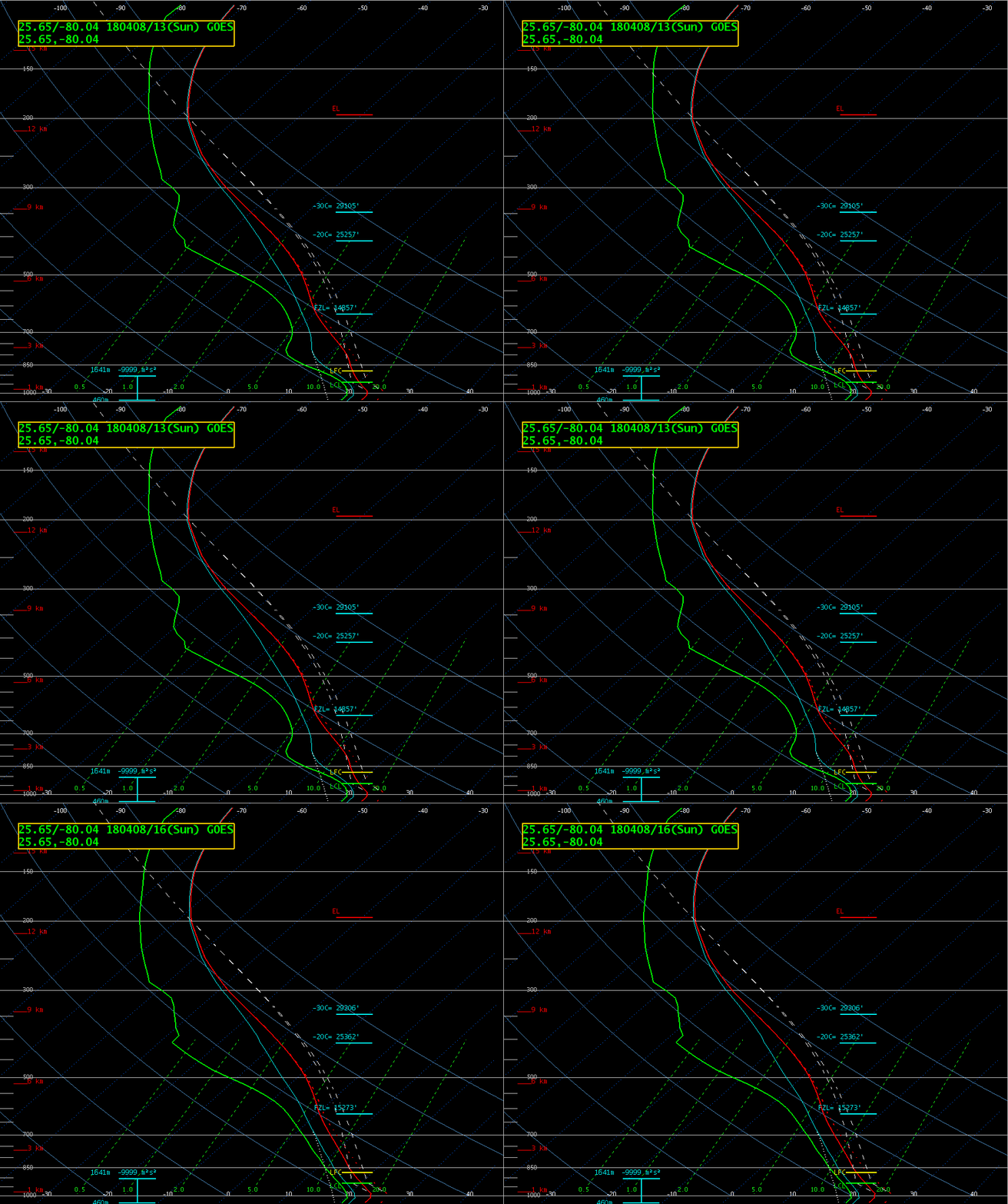
GOES-16 LAP Vertical Profiles of Temperature and Moisture at 13, 15 and 16 UTC for a point near Miami (Click to enlarge)
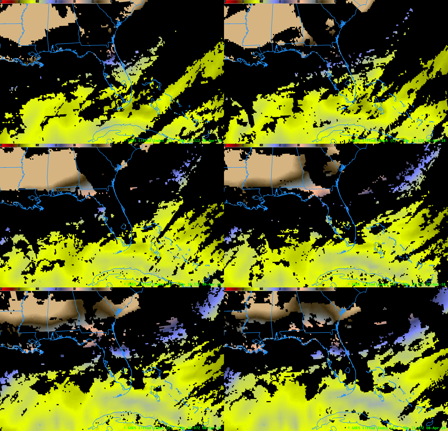
LAP data are used to create Derived Stability Indices (CAPE, Total Totals, Lifted Index, K-index, Showalter Index) and Total Precipitable Water. These integrated quantities, also available in AWIPS, are likely to be more useful to forecasters than point data. This is especially true because the most reliable information from the LAP Soundings and the derived stability indices are gradients and time tendencies. (Here is an animation of Lifted Index from 1332 – 2147 UTC on 8 April 2018)
In 2019, AWIPS will included gridded horizontal fields derived from NUCAPS temperature and moisture profiles. This will allow visualization of convective parameters such as Lifted Index and CAPE. In addition, NUCAPS soundings from NOAA-20 and from Metop-A and Metop-B will flow to AWIPS at some point after early Summer 2018, greatly increasing the number of observation-based soundings available.
View only this post
Read Less
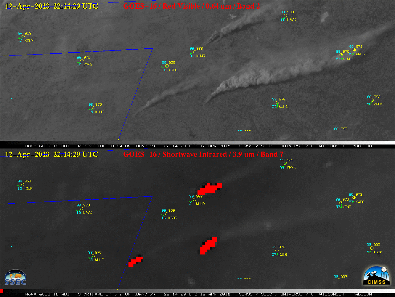
![SPC Day 1 Fire Outlook [click to enlarge]](https://cimss.ssec.wisc.edu/satellite-blog/wp-content/uploads/sites/5/2018/04/180412_spc_day1_fire_outlook.jpeg)
![Suomi NPP VIIRS Day/Night Band (0.7 µm) and Shortwave Infrared (3.9 µm) images [click to enlarge]](https://cimss.ssec.wisc.edu/satellite-blog/wp-content/uploads/sites/5/2018/04/180413_0837utc_suomi_npp_viirs_ShortwaveInfrared_DayNightBand_OK_fires_anim.gif)
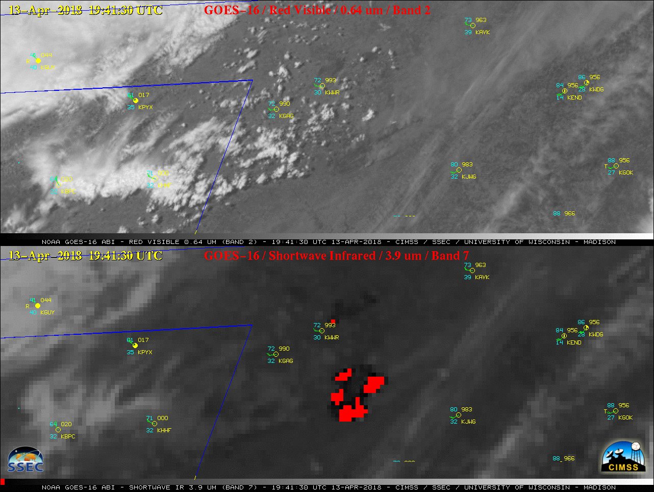
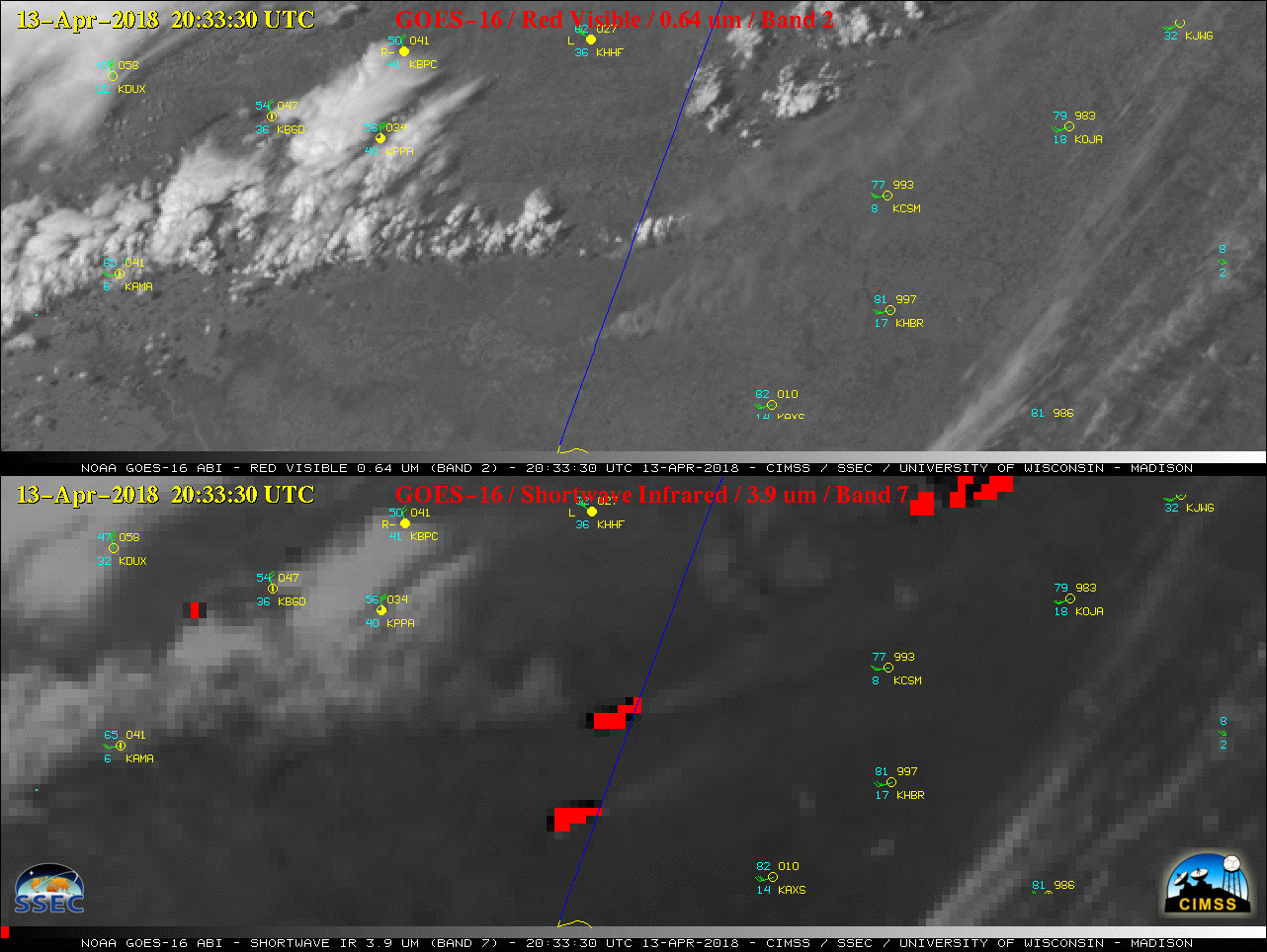
![NOAA-20 VIIRS Day/Night Band (0.7 µm) and Shortwave Infrared (3.75 µm) images at 0737 UTC [click to enlarge]](https://cimss.ssec.wisc.edu/satellite-blog/wp-content/uploads/sites/5/2018/04/180414_0737utc_viirs_DayNightBand_ShortwaveIR_NW_OK_fires_anim.gif)
![Suomi NPP VIIRS Day/Night Band (0.7 µm) and Shortwave Infrared (3.75 µm) images [click to enlarge]](https://cimss.ssec.wisc.edu/satellite-blog/wp-content/uploads/sites/5/2018/04/180414_0827utc_viirs_DayNightBand_ShortwaveIR_NW_OK_fires_anim.gif)
![NOAA-20 VIIRS Day/Night Band (0.7 µm) and Shortwave Infrared (3.75 µm) images [click to enlarge]](https://cimss.ssec.wisc.edu/satellite-blog/wp-content/uploads/sites/5/2018/04/180414_0917utc_viirs_DayNightBand_ShortwaveIR_NW_OK_fires_anim.gif)
![Terra MODIS true-color and false-color RGB images [click to enlarge]](https://cimss.ssec.wisc.edu/satellite-blog/wp-content/uploads/sites/5/2018/04/180415_1719utc_terra_modis_truecolor_falsecolor_northwestern_OK_fires_anim.gif)