This website works best with a newer web browser such as Chrome, Firefox, Safari or Microsoft
Edge. Internet Explorer is not supported by this website.
1-minute Mesoscale Domain Sector GOES-19 Infrared Window images (above) showed Tropical Storm Bertha as it moved slowly northwestward then westward across the far northern Gulf of Mexico on 21 July 2026. Pulses of overshooting tops exhibited infrared brightness temperatures in the -75 to -80 C range (brighter white pixels). 1-minute GLM Flash... Read More
1-minute GOES-19 Infrared Window images and GLM Flash Points, from 0301 UTC on 21 July to 0000 UTC on 22 July
1-minute Mesoscale Domain Sector GOES-19 Infrared Window images (above) showed Tropical Storm Bertha as it moved slowly northwestward then westward across the far northern Gulf of Mexico on 21 July 2026. Pulses of overshooting tops exhibited infrared brightness temperatures in the -75 to -80 C range (brighter white pixels). 1-minute GLM Flash Points displayed the lightning activity associated with deep convection near and south of the center of circulation.
1-minute GOES-19 Visible images (below) revealed that Bertha’s low-level circulation center (LLCC) remained partially to fully exposed during the day — since the tropical storm was moving through an environment characterized by high values of northeasterly deep-layer wind shear (1500 UTC | 2100 UTC), which acted to displace most of the deep convection south of the LLCC.
1-minute GOES-19 Visible images and GLM Flash Points, from 1141 UTC on 21 July to 0000 UTC on 22 July
===== 22 July Update =====
1-minute GOES-19 Visible images (left) and Infrared Window images (right), from 1101-1900 UTC on 22 July
1-minute GOES-19 Visible and Infrared Window images (above) showed that the fully-exposed eye of Tropical Storm Bertha made landfall in southeastern Louisiana at 1900 UTC on 22 July.
We are starting to see the onset of an active period of tropical development in the eastern Pacific basin. Over the weekend of 18-19 July 2026, two separate systems were experiencing different stages of their life: Elida was dying out near the west coast of Mexico while Fausto was starting... Read More
We are starting to see the onset of an active period of tropical development in the eastern Pacific basin. Over the weekend of 18-19 July 2026, two separate systems were experiencing different stages of their life: Elida was dying out near the west coast of Mexico while Fausto was starting to consolidate into a tropical storm. The following satellite loops from GOES-18 (GOES West) show these systems. The first is the Band 2 visible product. Elida is in the western center of the animation while Fausto is in the south central part of the loop.
Here’s the same loop as before, but from the Band 13 infrared perspective. Here, it is clear that Fausto represents deeper convection was the infrared imagery shows much colder cloud tops for that storm than it does for Elida.
Polar-orbiting satellites around this time provide some additional perspective on these storms. First, let’s look at some scatterometer data to evaluate near-surface winds. Here’s a view from OSCAT3 of Elida on Sunday the 19th. OSCAT tends to have more uncertainty in the wind vector retrievals than ASCAT does, but makes up for it with a wider swath and fewer gaps between swaths. (ASCAT was particularly unlucky with both storms on the 19th). Here we see clear evidence of a focused area of circulation with winds in the center maxing out at around 30-40 kts.
Going further south to Fausto at roughly the same time in the 19th, we see a circulation that is not quite as refined as Elida. Winds are slower and the center of circulation isn’t as circular.
Elida has propagated to the north, into the cooler waters of the midlatitude eastern Pacific. Between the 19th and the 20th, it lost its tropical storm status and is now officially post-tropical. However, Fausto is continuing to intensify and model tracks show that it may impact Hawaii in the coming days, so we’ll look at it a bit more. Here’s a frame from the CIMSS D-MINT product from 1930 UTC on the 19th, approximately the same time as the animated loops above). D-MINT uses microwave and infrared observations to assess the intensity of tropical cyclones. The left three panels show three different microwave channels, and forecasters can use these to more easily identify the center of circulation when the infrared or visible images are cluttered with high-level cirrus shields. Here we see the circulation is likely centered around the lower-left hand corner of the microwave images. The rightmost panel depicts the mean surface wind of the system as estimated by the D-MINT algorithm, and in this case it is around 30 kts.
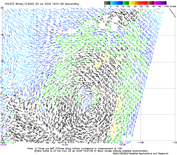
We can use satellites to gauge how much Fausto improved from Sunday the 19th into Monday the 20th. We’ll start by looking at more recent scatterometer observations. In the ~25 hours between the OSCAT plot shown above and the more recent one below, Fausto’s circulation tightened up immensely and became much more circular.
We also see the intensification in D-MINT. This prodcut relies on available microwave satellite observations and not all satellites contain the same set of channels, hence the difference in the images shown here. Regardless, the algorithm now projects a mean surface wind of 44 kts by 1524 UTC, about 20 hours later than the image above.
NOAA’s National Hurricane Center projects that Fausto will become a hurricane on the 20th. Model forecasts, including the GFS and Google’s DeepMind show Fausto continuing to the east-northeast, weaking to a tropical storm just before it passes to the north of Hawaii. However, the long-term forecasts also show additional Pacific tropical systems developing south of Mexico and continuing to the east, so eyes will be on the Pacific for some time to come.
Tropical Depression Two developed in the northeastern Gulf of Mexico at 1500 UTC on 19 July 2026 — and 1-minute Mesoscale Domain Sector GOES-19 (GOES-East) Visible images (above) showed the slow trend of organization during the day (there was a 49-minute gap in image coverage as Mesoscale Sectors were rearranged). GLM Flash... Read More
1-minute GOES-19 Visible images with an overlay of 1-minute GLM Flash Points, along with plots of Fixed Buoy (cyan) and Moving Maritime (yellow) reports, from 1141-2300 UTC on 19 July
Tropical Depression Two developed in the northeastern Gulf of Mexico at 1500 UTC on 19 July 2026 — and 1-minute Mesoscale Domain Sector GOES-19 (GOES-East) Visible images (above) showed the slow trend of organization during the day (there was a 49-minute gap in image coverage as Mesoscale Sectors were rearranged). GLM Flash Points highlighted intermittent lightning activity associated with areas of deep convection. Tropical Depression Two was moving very slowly through an environment of relatively low wind shear, and was traversing warm water.
Metop ASCAT surface scatterometer winds at 1424 UTC (below) were generally at or below 25 kts — and wind gusts from nearby buoys and ships were also 25 kts or less in the animation shown above.
GOES-19 Visible image at 1424 UTC on 19 July, with an overlay of Metop ASCAT winds [click to enlarge]
The corresponding 1-minute GOES-19 Infrared Window images (below) indicated that the coldest cloud-top infrared brightness temperatures of convection were generally in the -65 to -70 C range.
1-minute GOES-19 Infrared Window images with an overlay of 1-minute GLM Flash Points, along with plots of Fixed Buoy (cyan) and Moving Maritime (yellow) reports, from 1141-2300 UTC on 19 July
5-minute CONUS Sector GOES-18 (GOES-West) Visible and Infrared Window images (above) showed the rapid development of a relatively compact thunderstorm east-southeast of Salt Lake City on 18 July 2026. The coldest thunderstorm cloud-top infrared brightness temperature was -48.76 C at 1741 UTC (above) — which represented an altitude just below the Most... Read More
5-minute GOES-18 Visible images (left) and Infrared Window images (right), from 1536-1831 UTC on 18 July
5-minute CONUS Sector GOES-18 (GOES-West) Visible and Infrared Window images (above) showed the rapid development of a relatively compact thunderstorm east-southeast of Salt Lake City on 18 July 2026.
Cursor sample of the coldest cloud-top infrared brightness temperature at 1741 UTC on 18 July [click to enlarge]
The coldest thunderstorm cloud-top infrared brightness temperature was -48.76 C at 1741 UTC (above) — which represented an altitude just below the Most Unstable (MU) air parcel’s Equilibrium Level (EL), according to a plot of 1800 UTC rawinsonde data from Salt Lake City (below).
Plot of rawinsonde data from Salt Lake City at 1800 UTC on 18 July [click to enlarge]
This thunderstorm produced GOES-18 GLM-detected lightning activity from 1726-1816 UTC (below) — beginning 5 minutes after the LightningCast probability first exceeded 75% (violet contours), and 10 minutes after the probability first exceeded 50% (green contours). The parallax-adjusted LightningCast product was used in this case, to portray the highest probability of lightning at the surface (instead of at the cloud top). Tragically, a hiker died after being struck by lightning near American Fork Twin Peaks (which is located about 4 miles southwest of Alta). (media report)
5-minute GOES-18 Visible images (left) and Infrared Window images (right) with overlays of GLM Flash Extent Density, GLM Flash Points and LightningCast Probability, from 1536-1831 UTC on 18 July
A time series of GOES-18 LightningCast probability and GLM flash counts in the vicinity of Heber City Municipal Airport (KHCR) — the closest airport to the fatal lightning event — is shown below. In addition, at 1756 UTC lightning in the distance was noted at Salt Lake City (KSLC) and Provo (KPVU).
Time series of GOES-18 LightningCast probability (pink) and GLM flash counts (blue dots) within 8 miles of Heber City Municipal Airport (KHCR), from 1601-1831 UTC on 18 July [click to enlarge]
The largest GOES-18 GLM Flash Point area in the vicinity of Alta was 228 km2 at 1806 UTC (below). Note that the Flash Point appeared just south of the cluster of large Flash Extent Density pixels — this is because gridded GLM products (such as Flash Extent Density) are mapped to correspond to a mean cloud top height, in contrast to the Flash Points which are mapped to correspond to the surface location of the lightning.
Cursor sample of GOES-18 GLM Flash Extent Density and GLM Flash Point at 1806 UTC on 18 July [click to enlarge]
This is the fifth known U.S. lightning fatality of 2026 and the first in Utah since August 2024. 13 hikers have been killed by lightning since 2006. Know the forecast before your hike and head to a safe place when you see building clouds or hear thunder!kutv.com/news/local/h…


