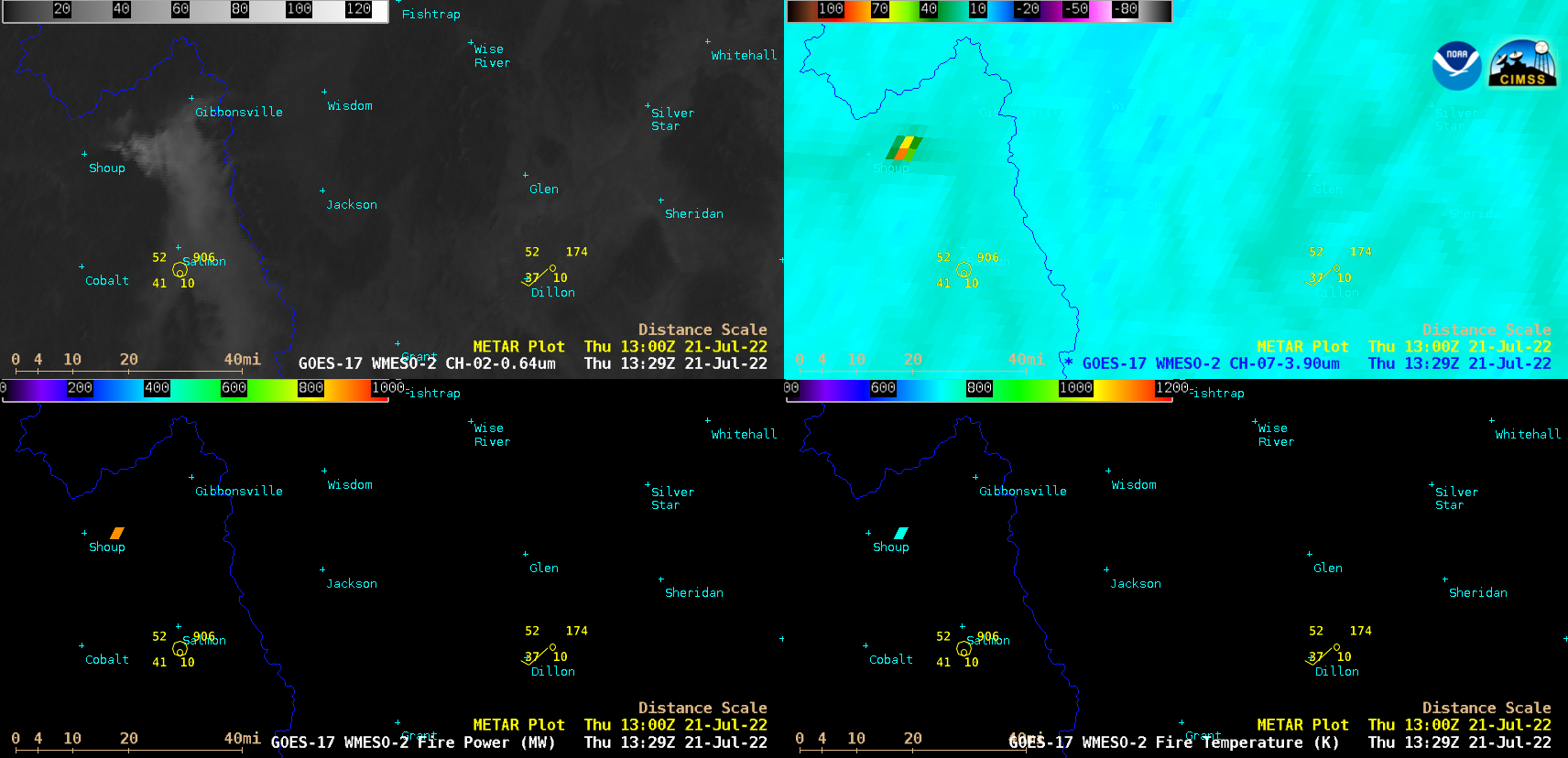
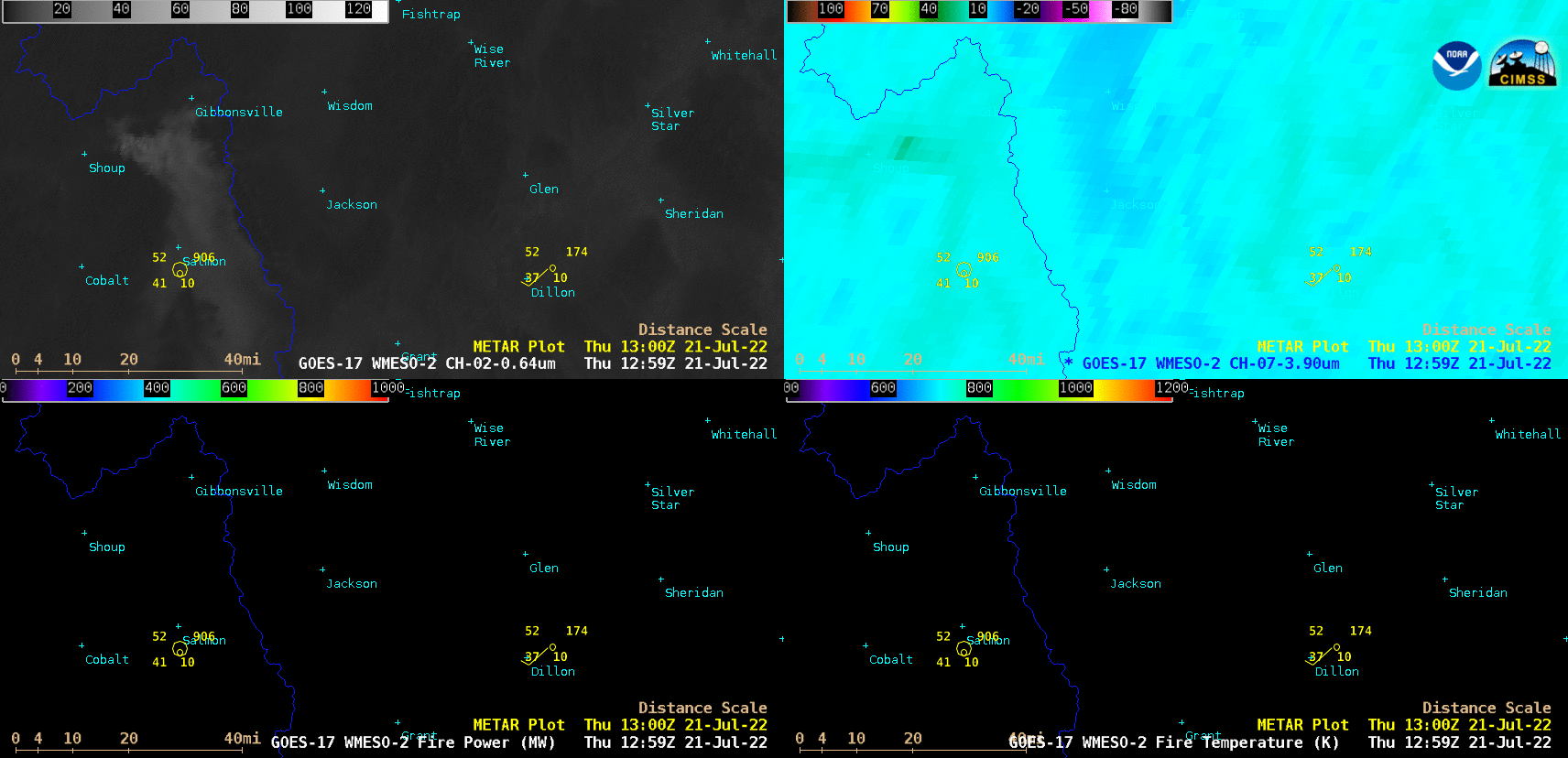
This website works best with a newer web browser such as Chrome, Firefox, Safari or Microsoft
Edge. Internet Explorer is not supported by this website.
1-minute Mesoscale Domain Sector GOES-16 (GOES-East) “Red” Visible (0.64 µm) images (above) include time-matched SPC Storm Reports — and showed some of the widespread severe weather produced by thunderstorms that developed ahead of a cold front which was moving eastward across the Deep South on 22 March 2022. The severe weather persisted for several hours past... Read More
GOES-16 “Red” Visible (0.64 µm) images, with time-matched SPC Storm Reports plotted in red [click to play animated GIF | MP4]
1-minute Mesoscale Domain Sector GOES-16 (GOES-East) “Red” Visible (0.64 µm) images (above) include time-matched SPC Storm Reports — and showed some of the widespread severe weather produced by thunderstorms that developed ahead of a cold front which was moving eastward across the Deep South on 22 March 2022.
The severe weather persisted for several hours past sunset, as displayed below by GOES-16 “Clean” Infrared Window (10.35 µm) images ending at 0416 UTC on 23 March (11:16 pm CDT on 22 March).
GOES-16 “Clean” Infrared Window (10.35 µm) images, with time-matched SPC Storm Reports plotted in blue [click to play animated GIF | MP4]
A closer look at the development of a supercell thunderstorm that produced an EF-3 tornado in Arabi (within the eastern portion of the Greater New Orleans metropolitan area) is shown below.
GOES-16 “Clean” Infrared Window (10.35 µm) images, with time-matched SPC Storm Reports plotted in blue [click to play animated GIF | MP4]
Tuesday's EF-3 tornado had an est. peak wind of 160 mph, making it the strongest tornado to impact Orleans/Jefferson/St. Bernard Parishes on record. It's also only the second F-/EF-3 or higher tornado. A small section of New Orleans East were impacted by both EF-3 tornadoes. pic.twitter.com/IlEFLjLHGq
Severe weather season is underway across the southern U.S. NOAA and CIMSS are using satellite, radar, and lightning observations of thunderstorms to develop and evaluate artificial intelligence (AI) tools that forecast and diagnose convection.The NOAA/CIMSS ProbSevere portfolio has several such tools to help forecasters keep tabs on storms. LightningCastProbSevere LightningCast... Read More
Severe weather season is underway across the southern U.S. NOAA and CIMSS are using satellite, radar, and lightning observations of thunderstorms to develop and evaluate artificial intelligence (AI) tools that forecast and diagnose convection.The NOAA/CIMSS ProbSevere portfolio has several such tools to help forecasters keep tabs on storms.
LightningCast
ProbSevere LightningCast is a model that uses images of geostationary ABI data from GOES-16 or GOES-17 to predict where lightning will strike (as observed by the GLM) out to 60 minutes. We’ve found that the product frequently provides 15-30 minutes of lead-time to lightning initiation, measured from the 30-40% probability range (the most skillful range). LightningCast will be evaluated at the 2022 NOAA Hazardous Weather Testbed and at certain offices within the NWS. LightningCast may be able to one day aid forecasters in providing decision support services and general convective initiation situational awareness. Below is a movie of LightningCast output (contours) overlaid on the GOES-16 daytime cloud phase distinction RGB and GLM flash-extent density, for the developing severe storms in Texas on March 21st.
IntenseStormNet
Another image-based AI model within ProbSevere is called IntenseStormNet, which seeks to identify the most intense regions of thunderstorms. It uses images of ABI and GLM data as predictors to probabilistically diagnose storm intensity from a geostationary perspective. Its goal is to identify intense parts of storms as humans do: holistically; by picking up on the spatial and multispectral features that imagery captures, such as overshooting tops, cold-U/AACP, cloud-top texture patterns, and stark cloud edges. In a paper published in 2020, we found that high probabilities from IntenseStormNet are frequently correlated with severe weather reports. Below shows IntenseStormNet output (contours) for some of the storms over Texas on March 21st, most of which spawned hail, damaging winds, and several tornadoes. IntenseStormNet contours can also be tracked over time, providing a novel way to investigate convective properties of storms.
ProbSevere v3
IntenseStormNet output is also being used as a predictor within the experimental ProbSevere v3, which uses satellite, radar, lightning, and NWP data, and machine-learning (ML) models to forecast the probabilities of hail, severe winds, and tornadoes in the next 60 minutes. While ProbSevere v2 is operational at NOAA’s Centers for Environmental Prediction, ProbSevere v3 is being evaluated by NWS forecasters at the 2022 Hazardous Weather Testbed. An analysis of thousands of storms from 2021 showed that additional predictors and the more sophisticated ML models in v3 improve upon v2 performance. ProbSevere uses multi-sensor storm tracking and feature extraction to predict probabilities of severe weather across the U.S. Below are several animations of ProbSevere v3 output in Texas on March 21st.
ProbSevere v3 output (contours), MRMS composite reflectivity, and NWS severe weather warnings for storms in northern Texas on March 21st.ProbSevere v3 output (contours), MRMS composite reflectivity, and NWS severe weather warnings for storms in central Texas on March 21st.
The image below shows GOES-16 Fire Power, a Fire Detection/Characterization Algorithm (FDCA) output field (along with Fire Temperature and Fire Area), on a day when strong southerly winds helped support multiple fires over Texas (as shown in this animation, from this blog post). If you do not have access to AWIPS, as below... Read More
The image below shows GOES-16 Fire Power, a Fire Detection/Characterization Algorithm (FDCA) output field (along with Fire Temperature and Fire Area), on a day when strong southerly winds helped support multiple fires over Texas (as shown in this animation, from this blog post). If you do not have access to AWIPS, as below (or in the linked-to animation), are there other ways to access and display FDCA output? This blog post shows how to do that with McIDAS-V.
GOES-16 Fire Power, 2101 UTC on 20 March 2022 (click to enlarge)
Where can you get the FDCA data to display? The NOAA CLASS data respository is one place. The toggle below outlines the products to choose in the drop-down menu (“GOES-R Series ABI Products (GRABIPRD) partially restricted L1b and L2+ Data Products”) near the top of the CLASS home page (then click on the >>GO), and then shows how to select the data wanted. In the example below, I’ve chosen the ABI L2+ GOES-16 CONUS files of Fire/Hot Spot Characterization on 20 March 2022 between 21:00 and 21:04. After making those selections, click on ‘Search’ and then order. When the files are queued up for retrieval, you’ll receive an email with instructions.
NOAA CLASS website, and GOES-R L2 Products data selection (Click to enlarge)
You can also access GOES-R data through this website below hosted at the University of Utah. (Kudos to Brian Blaylock, its developer!) Note in the animation below how you choose the satellite, the product and the time, and then receive a list of downloadable files.
Amazon Web Services portal showing data selection and files retrieved (Click to enlarge)
You can start up McIDAS-V to view the data once you have downloaded to your machine the data file:
FDCC in the filename signifies Fire Detection Characterization in the CONUS domain, created with Mode 6 scanning (M6) and GOES-16 data (G16). The data starts at 21:01:16.8 on 20 March (Julian Day 79) in 2022, i.e., 20220792101168 and ends at 21:03:54.1 on the same day. It was created at 21:04:15.5. Once you start McIDAS-V, you must input the data, via the Data Sources tab within the Data Explorer. The satellite data we’re using are gridded data, and they’re local. Select the file needed for display and click ‘Add Source’. When you do that, you’ll see a different window (‘Field Selector’) brought to the front.
McIDAS-V Data Explorer (Click to enlarge)Steps under ‘Field Selector’ in the Data Explorer to find the data to display (Click to enlarge)
Note in this example that 5 different fields are present in the file: Fire + Hot Spot Characterization Fire Area, Fire Temperatures, Fire Mask, Fire Radiative Power and Data Quality Flags. In this example, I’ve selected ‘Data Quality Flags’ — to be presented as ‘Value Plots’; those are shown below in a region zoomed in over Texas and annotated.
FDCA Data Quality Flags, 2101 UTC, 20 March 2022 (Click to enlarge)
Rather than Data Quality Flags, one can show ‘Fire Mask’ — these data values are available in AWIPS files, but aren’t generally shown. So, I recreated the ‘Value Plots’ but selected ‘Fire Mask’ rather than ‘data quality Flags’; Next, I created a ‘Color-Shaded Plan View’ (the Data Explorer for that is shown here, created with ‘Match Display Region’ chosen). The animation below steps through the plotted values, the color-shaded plan view with default enhancement, and the color-shaded plan view with a McIDAS Enhancement Table appropriate to the Fire Mask (clouds, for example, are grey, and fires stand out against the background). (This pdf describes what the file mask values mean).
Plotted FDCA Fire Mask values, and color-enhanced gridded values, 2101 UTC on 20 March 2022 (click to enlarge)
This toggle compares Fire Mask, and Fire Power. A zoom in on Fire Power to north Texas, below, shows the same data as the AWIPS screen grab at the top of this blog post. They are nearly identical.
GOES-16 FDCA Fire Power, 2101 UTC on 20 March 2022 (click to enlarge)
Use McIDAS-V to display Level 2 products if it is difficult to find them online.
As noted here, an updated version of geo2grid is being prepared at CIMSS. As part of that upgrade, support for some level 2 products will be included. For example, the image above — of cloud-top height — was created using the following set of geo2grid (a beta version that this... Read More
Cloud-top Height, 1510 UTC on 21 March 2022 (click to enlarge)
As noted here, an updated version of geo2grid is being prepared at CIMSS. As part of that upgrade, support for some level 2 products will be included. For example, the image above — of cloud-top height — was created using the following set of geo2grid (a beta version that this blogger is testing) calls.
How does the image above compare to Level 2 product fields that can be found elsewhere? This website contains a link to a RealEarth instance that includes mappings of Full-Disk Cloud Mask, Cloud Top Pressure, Cloud top Phase, and Cloud Optical Depth. A portion of the Full-Disk Cloud Top Pressure is shown below (from 1500 UTC). Similar features are apparent in fields above and below.
GOES-16 Cloud Top Pressure, 1500 UTC on 21 March 2022 (click to enlarge)
Level 2 Products associated with Cloud-top properties are also available at the CIRA slider, including Cloud-top Height, shown below from 1501 UTC. Other GOES-R Level 2 products available there include Cloud Optical Depth, Cloud Mask, Cloud Phase and Cloud Effective Particle Size.
GOES-16 Cloud-top Height, 1501 UTC on 21 March 2022 (click to enlarge)