GOES-16 “Clean” Infrared Window (10.35 µm) images, with hourly precipitation type symbols plotted yellow and Interstates plotted in gray [click to play animated GIF | MP4]
GOES-16 (GOES-East) “Clean” Infrared Window (10.35 µm) images (above) showed the development of an elongated band of training thunderstorms that was responsible for producing record rainfall and flash flooding in the St. Louis, Missouri area during the nighttime hours leading up to sunrise on 26 July 2022. The coldest GOES-16 cloud-top infrared brightness temperatures were around -75ºC.
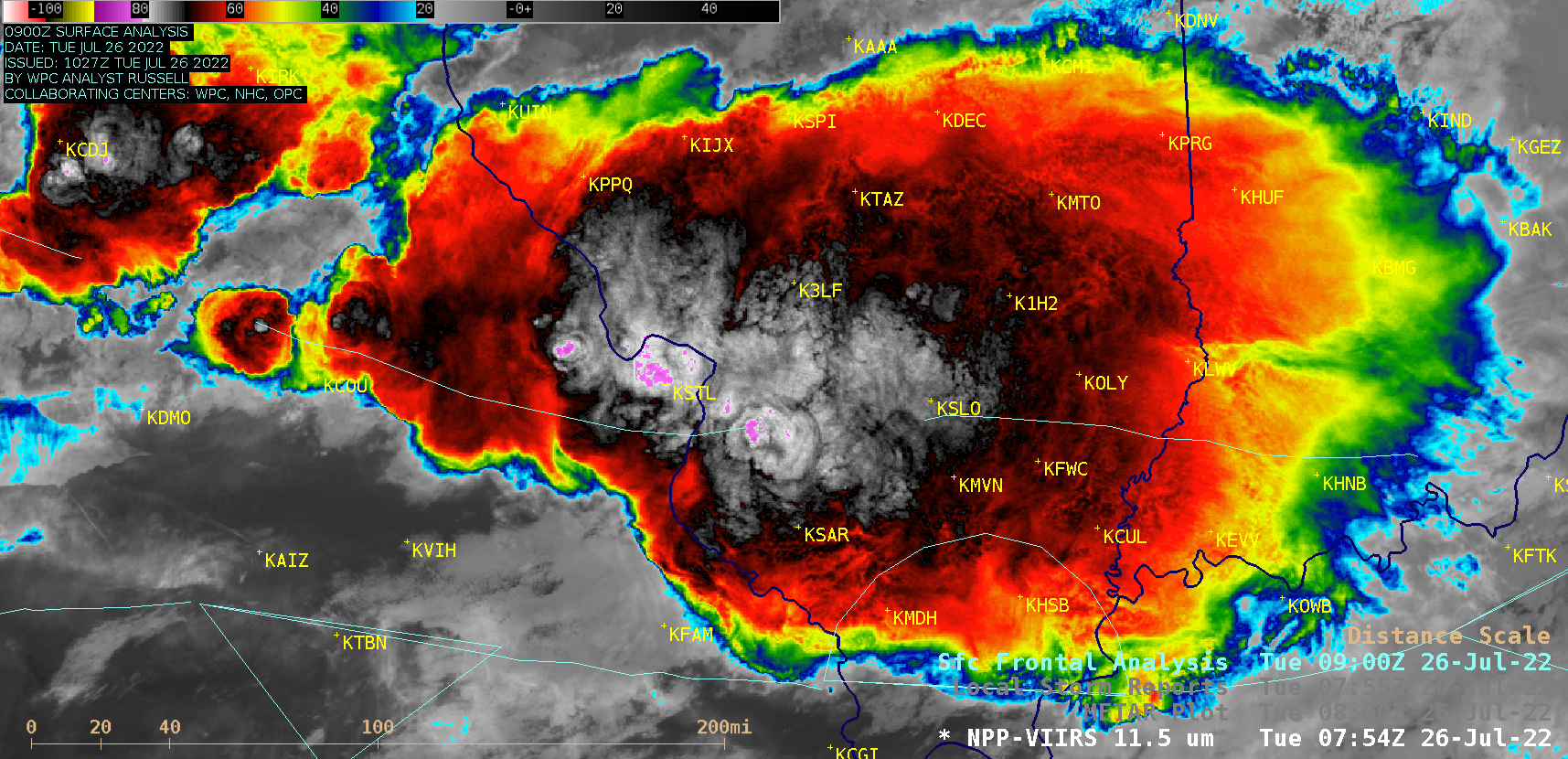
A Suomi-NPP VIIRS Infrared Window (11.45 µm) image valid at 0802 UTC (below) displayed the large Mesoscale Convective System as it was just beginning to move away from the St. Louis (KSTL) area. The coldest cloud-top infrared brightness temperature in the VIIRS image was -83ºC (within the interior shades of violet). These thunderstorms developed as a southwesterly low-level jet began to increase isentropic upglide across and north of a stationary front that was located just south of the deep convection (surface analyses | WPC Mesoscale Precipitation Discussion).
Suomi-NPP VIIRS Infrared Window (11.45 µm) image valid at 0802 UTC [click to enlarge]
View only this post Read Less


