This website works best with a newer web browser such as Chrome, Firefox, Safari or Microsoft
Edge. Internet Explorer is not supported by this website.
GOES-16 (GOES-East) “Red” Visible (0.64 µm), Shortwave Infrared (3.9 µm) and “Clean” Infrared Window (10.35 µm) images (above) showed that a large wildfire burning in far western Manitoba produced a series of 3 brief pyrocumulonimbus (pyroCb) clouds late in the day on 19 July 2022. The coldest pyroCb cloud-top infrared brightness temperature was -52.1ºC at 0230 UTC.GOES-18 images... Read More
GOES-16 “Red” Visible (0.64 µm, top), Shortwave Infrared (3.9 µm, center) and “Clean” Infrared Window (10.35 µm, bottom) images [click to play animated GIF | MP4]
GOES-16 (GOES-East) “Red” Visible (0.64 µm), Shortwave Infrared (3.9 µm) and “Clean” Infrared Window (10.35 µm) images (above) showed that a large wildfire burning in far western Manitoba produced a series of 3 brief pyrocumulonimbus (pyroCb) clouds late in the day on 19 July 2022. The coldest pyroCb cloud-top infrared brightness temperature was -52.1ºC at 0230 UTC.
GOES-18 images shown in this blog post are preliminary and non-operational
In the corresponding imagery from GOES-18, the coldest pyroCb cloud-top infrared brightness temperature was -53.3ºC at 0230 UTC.
GOES-18 “Red” Visible (0.64 µm, top), Shortwave Infrared (3.9 µm, center) and “Clean” Infrared Window (10.35 µm, bottom) images [click to play animated GIF | MP4]
In a previous post, we explored a data interpolation technique that involved running sections of missing GOES-17 Band 13 data through a shape-preserving piecewise cubic spline method in order to fill the data gaps for brightness temperature (BT). (That method was nicknamed ‘pchip’ interpolation.) In this post, we introduce a more... Read More
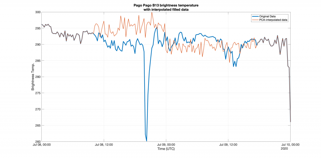
In a previous post, we explored a data interpolation technique that involved running sections of missing GOES-17 Band 13 data through a shape-preserving piecewise cubic spline method in order to fill the data gaps for brightness temperature (BT). (That method was nicknamed ‘pchip’ interpolation.) In this post, we introduce a more advanced type of interpolation for data filling known as interpolation by Principal Component Analysis, or PCA interpolation. One benefit of PCA interpolation is that data does not need to be smoothed to create a believable interpolation. It is, however, more computationally intense and the interpolation requires more time.
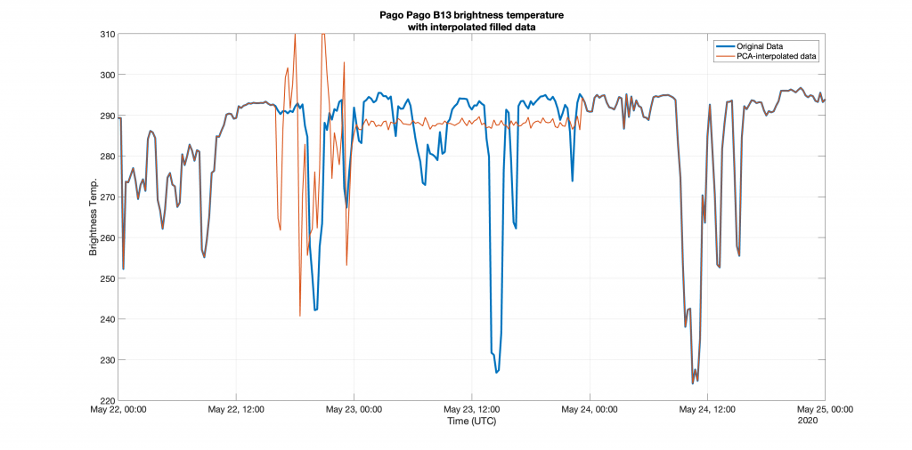
To test PCA interpolation, artificial gaps are created in portions of the complete GOES-17 time series data and compared for accuracy. The longest real gap in the GOES-17 time series is approximately 31 hours. Twenty artificial gaps of 31 hours are created in the time series and run through PCA interpolation. Examples are shown below.
Example 1 of PCA-filled data (red) compared to the original true data (blue) for 31 hours of data on May 22, 2020. The red line is an interpolation or ‘educated guess’ of the blue line values, using Principal Component Analysis.Example 2 of PCA-filled data (red) compared to the original true data (blue) for 31 hours of data on July 8, 2020. The red line is an interpolation or ‘educated guess’ of the blue line values, using Principal Component Analysis.
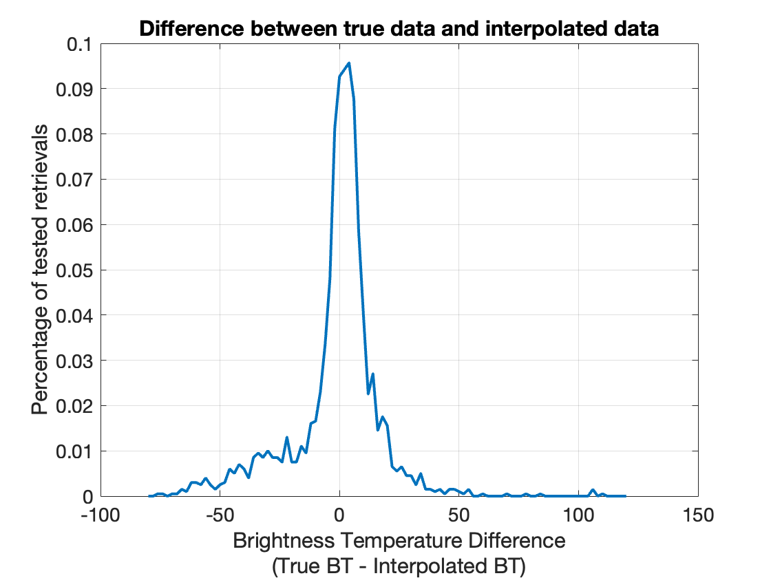
Clearly from the examples above, the PCA interpolation does not replicate the original data. Comparing the trends by eye, the PCA interpolation does not seem to mimic the original data well. However, the difference between the true BT and the interpolated BT is computed and has a mean of 1.2032 Kelvin, which is fairly low. 51.4% of all tested retrievals yielded a difference of less than 10 Kelvin. That is, for more than half of the tested retrievals, the filled interpolation is within 10 Kelvin of the original value.
A distribution of the differences between interpolated BT and true BT for the retrievals tested.
The animation above shows ACSPO estimates of Lake Surface Temperature (LST) over Lake Michigan from 3 different VIIRS overpasses: NPP at 0703 and 0844, and NOAA-20 at 0753 UTC (despite the AWIPS label!) early on 18 July 2022; VIIRS data were downloaded at the CIMSS Direct Broadcast antennae, and ACSPO... Read More
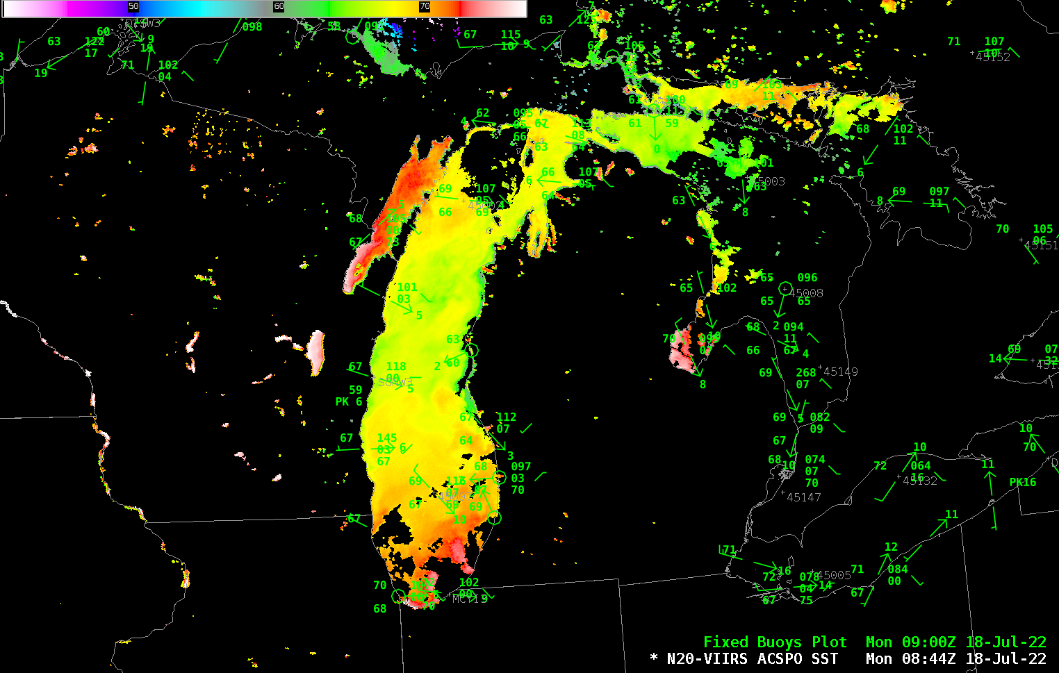
VIIRS ACSPO SSTs, 0703, 0753 and 0844 UTC on 18 July 2022, along with buoy observations (Click to enlarge)
The animation above shows ACSPO estimates of Lake Surface Temperature (LST) over Lake Michigan from 3 different VIIRS overpasses: NPP at 0703 and 0844, and NOAA-20 at 0753 UTC (despite the AWIPS label!) early on 18 July 2022; VIIRS data were downloaded at the CIMSS Direct Broadcast antennae, and ACSPO SST fields were created using CSPP software; AWIPS-ready tiles are available via an LDM feed from CIMSS. Orange to red enhancement values show lake surface temperature at/above 20oC/68oF (the color bar limits are 41oF/77oF). Two NOAA buoys are also present within Lake Michigan, and both show lake temperatures of 69oF; satellite values show far greater variability within the lake than can be deduced from just two buoy-based observations.
GOES-R data are used to create lake-surface (and sea-surface) temperatures. The toggle below over Green Bay and central Lake Michigan shows the superior spatial resolution of the VIIRS instrument. Over the open lake, GOES-R SSTs run about 1/2oF warmer than SSTs from VIIRS.
GOES-16 and VIIRS SST estimates over Green Bay and central Lake Michigan, ca. 0900 UTC on 18 July 2022 (click to enlarge)
Similar imagery (also using Direct Broadcast data and created using CSPP software) was available slightly later off the coast of Oregon, as shown below. Three consecutive passes of VIIRS, at about 45-minute intervals, allow for changes in the surface temperature fields to be monitored with high spatial and temporal resolution.
VIIRS ACSPO SSTs, 0934, 1026 and 1118 UTC on 18 July 2022 (Click to enlarge)
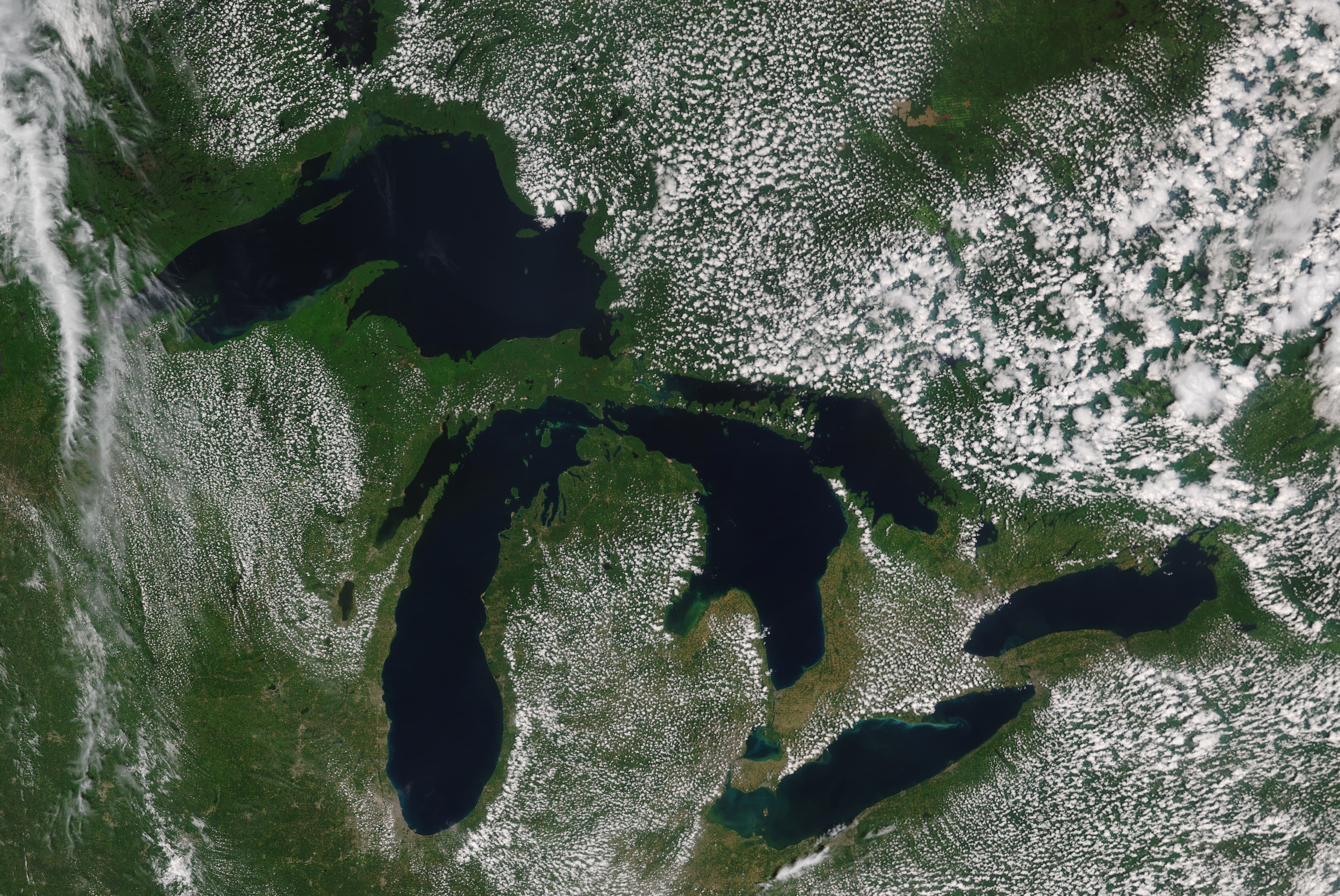
ACSPO SST (and individual channel, and true/false color) imagery is routinely available at the CIMSS direct broadcast site at this link for NOAA-20 and this link for NPP. You can also find True Color imagery over the Great Lakes, such as the image below from NOAA-20, posted for your viewing pleasure.
NOAA-20 True-Color imagery over the Great Lakes, 1850 UTC on 14 July 2022 (Click to enlarge)
GOES-18 images shown in this blog post are preliminary and non-operational Overlapping 1-minute Mesoscale Sectors provided 30-second images of GOES-18 “Red” Visible (0.64 µm) data, which showed the circulation of a Mesoscale Convective Vortex (MCV) that moved northward across southern Nevada early in the day on 17 July 2022. Ongoing thunderstorms along the periphery... Read More
GOES-18 “Red” Visible (0.6.4 .µm) images [click to play animated GIF | MP4]
GOES-18 images shown in this blog post are preliminary and non-operational
Overlapping 1-minute Mesoscale Sectors provided 30-second images of GOES-18 “Red” Visible (0.64 µm) data, which showed the circulation of a Mesoscale Convective Vortex (MCV) that moved northward across southern Nevada early in the day on 17 July 2022. Ongoing thunderstorms along the periphery of this MCV slowly dissipated as they moved across California and Nevada — and according the morning NWS Las Vegas forecast discussion, some of these storms produced rare July rainfall in parts of Death Valley, California.
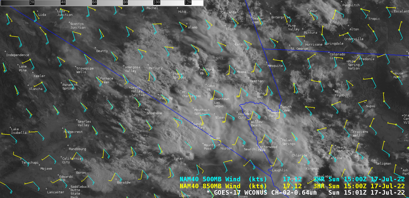
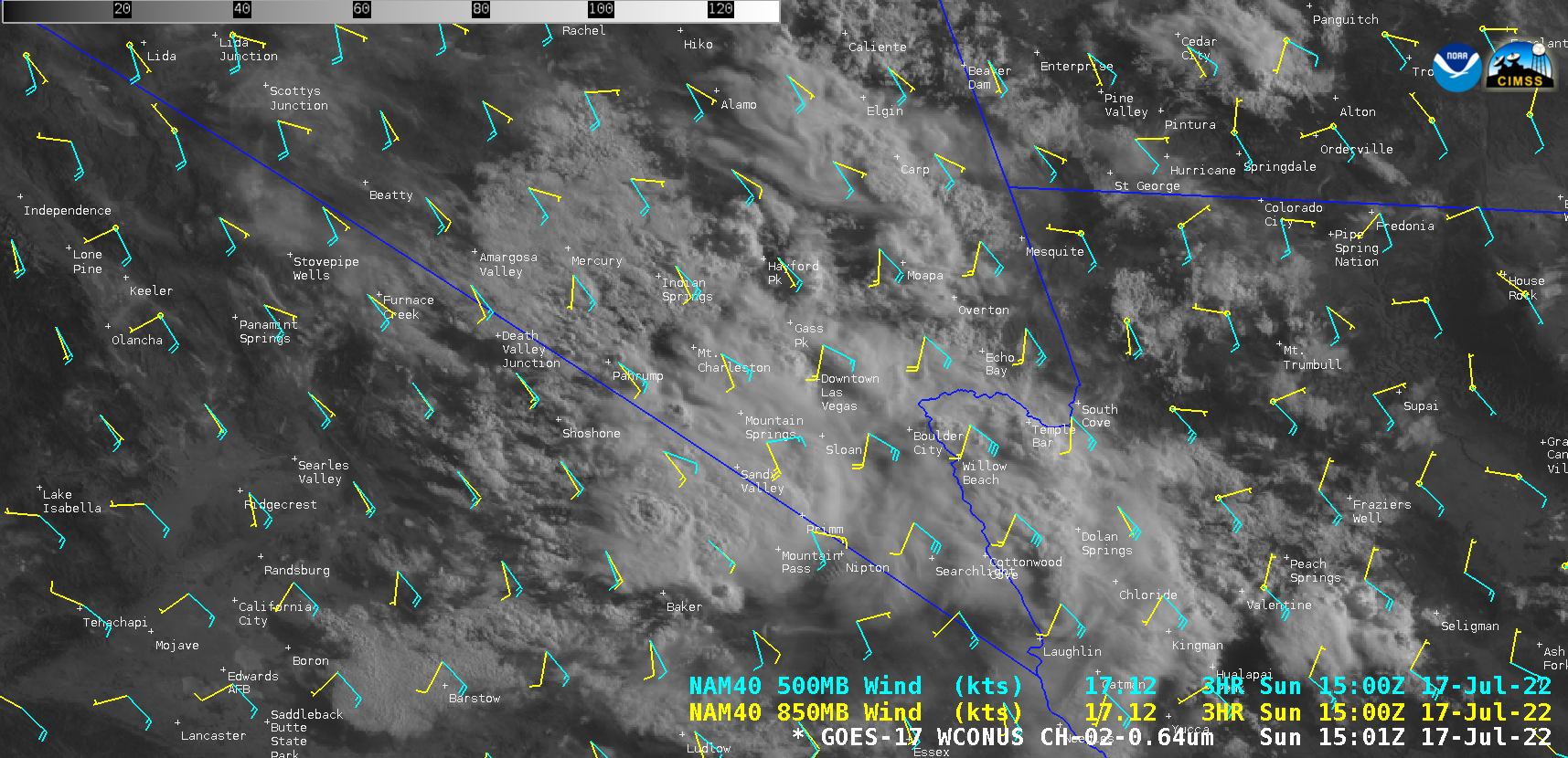
According to NAM40 model winds, this MCV was moving through an environment of generally low wind shear (below), where there was also sufficient moisture and instability.
GOES-17 “Red” Visible (0.6.4 .µm) image, with plots of NAM40 model 850 hPa and 500 hPa wind barbs [click to enlarge]
The GOES-18 Total Precipitable Water (source) derived product (below) also showed abundant moisture across much of the Desert Southwest as the MCV approached — which helped to sustain the MCV as it moved across southern Nevada.
GOES-18 Total Precipitable Water derived product [click to play animated GIF | MP4]


