
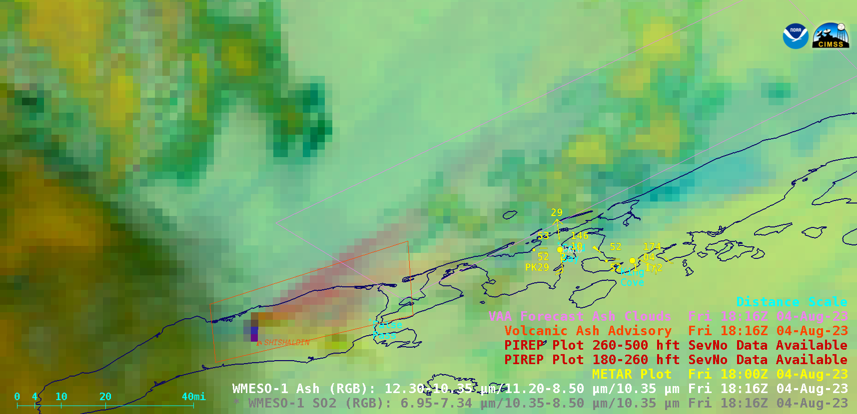
GOES-18 (GOES-West) Ash RGB images (above) showed the northeastward drift of volcanic clouds produced by an eruption of Mount Shishaldin that began just before 1300 UTC on 04 August 2023 (a Mesoscale Domain Sector was positioned over that region at 1603 UTC, providing 1-minute imagery after that time). Those northeast-moving volcanic clouds contained moderate concentrations of ash (denoted... Read More
GOES-18 Ash RGB and SO2 RGB images [click to play animated GIF | MP4]
GOES-18
(GOES-West) Ash RGB images
(above) showed the northeastward drift of volcanic clouds produced by an eruption of
Mount Shishaldin that began just before 1300 UTC on 04 August 2023 (a
Mesoscale Domain Sector was positioned over that region at 1603 UTC, providing 1-minute imagery after that time). Those northeast-moving volcanic clouds contained moderate concentrations of ash (denoted by shades of pink in the Ash RGB images) — then after 1700 UTC,
SO2 RGB images revealed the formation of a southeast-moving volcanic cloud that contained modest concentrations of SO2 (shades of yellow) that drifted just to the south of False Pass (in the SO2 RGB images, the northeast-moving ash clouds exhibited darker shades blue). High clouds began to overspread the area from the west after 1830 UTC, which tended to mask the volcanic signatures.
1-minute GOES-18 True Color RGB images from the CSPP GeoSphere site (below) helped to highlight the ash-rich volcanic cloud (shades of tan to brown) moving northeast from the summit of Shishaldin, and also showed the higher-altitude volcanic cloud drifting southeast (which contained SO2).
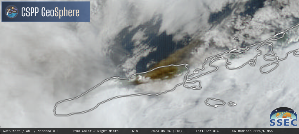
GOES-18 True Color RGB images [click to play MP4 animation]
A plot of 0000 UTC rawinsonde data from Cold Bay, Alaska
(below) indicated that northwesterly winds existed at altitudes of 28000 ft (9 km) and higher, with southwesterly winds below that level (down to altitudes around 20000 ft or 6 km).
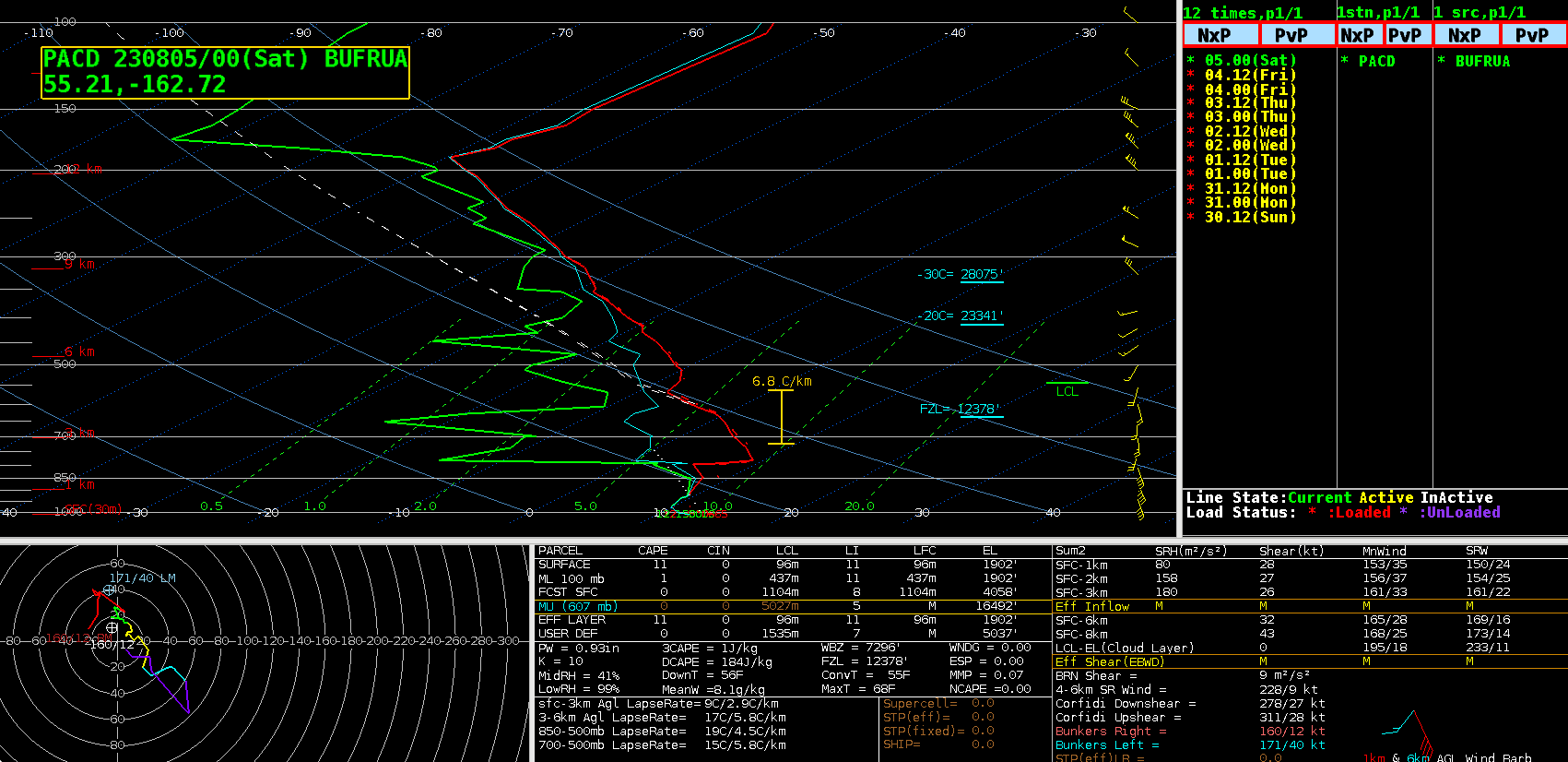
Plot of 0000 UTC rawinsonde data from Cold Bay, Alaska [click to enlarge]
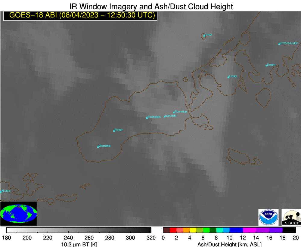
Radiometrically-retrieved GOES-18 Ash Cloud Height from the
NOAA/CIMSS Volcanic Cloud Monitoring site
(below) showed that maximum height values were generally in the 6-8 km (20000-26000 ft) range.
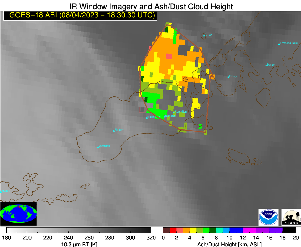
GOES-18 Ash Cloud Height [click to play animated GIF | MP4]
Given that volcanic ash presents a significant hazard to aviation, Volcanic Ash Advisories and Forecasts were issued
(below).
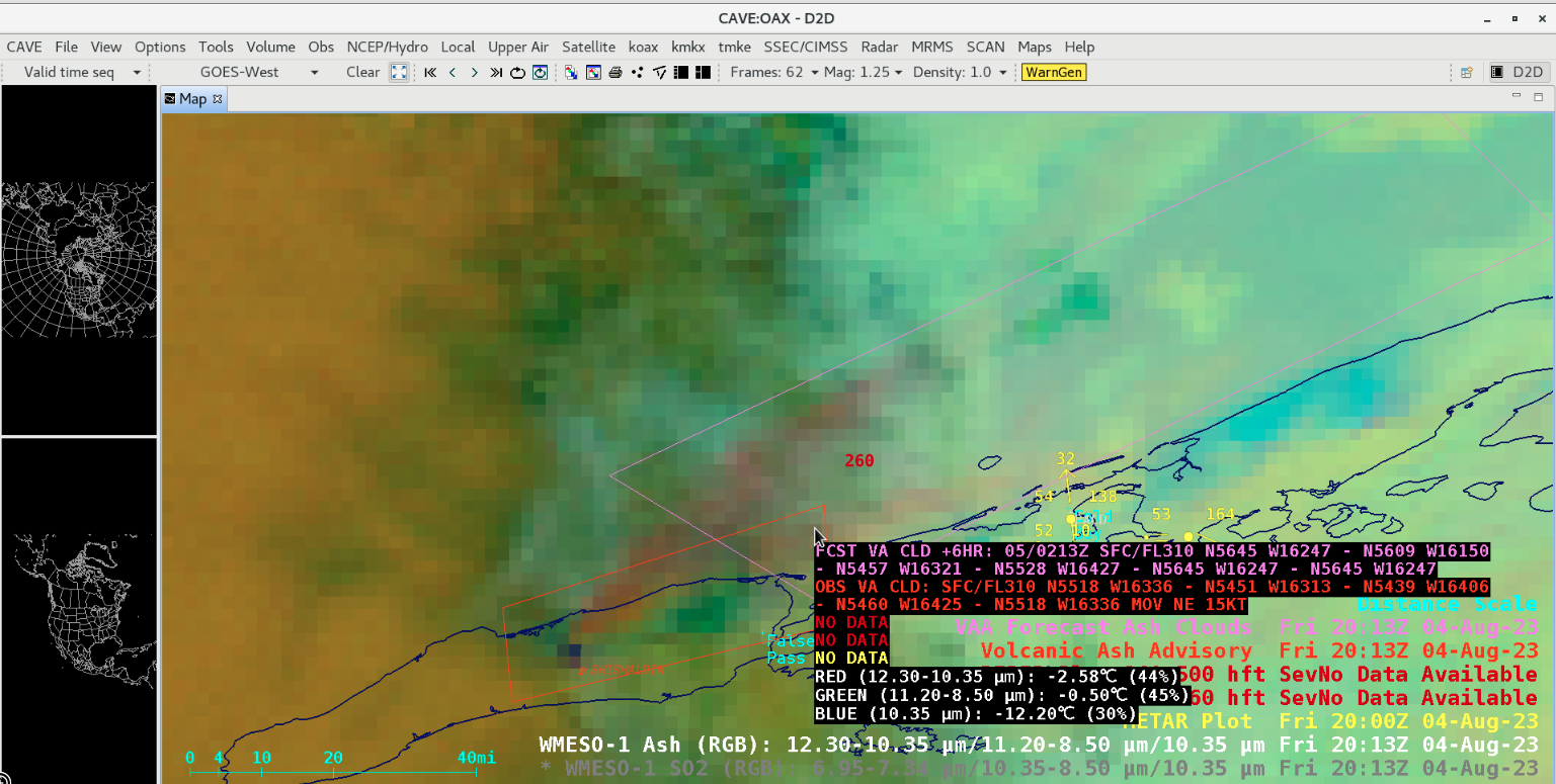
GOES-18 Ash RGB image, with Volcanic Ash Advisory (red) and Forecast (violet) polygons issued at 2013 UTC [click to enlarge]
GOES-18 Ash RGB images with a few Pilot Reports that mentioned the altitude of volcanic ash are shown below.
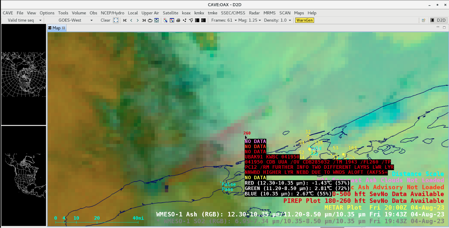
Pilot Report at 1943 UTC, mentioning ash at two different altitudes (moving in different directions) [click to enlarge]
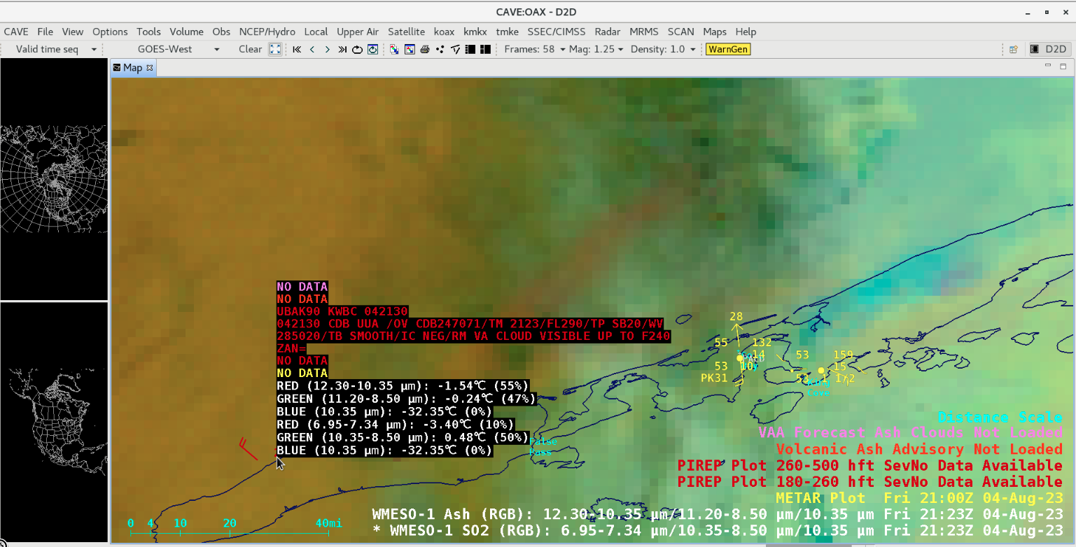
Pilot Report at 2123 UTC, describing volcanic ash (VA) up to an altitude of 24000 ft [click to enlarge]
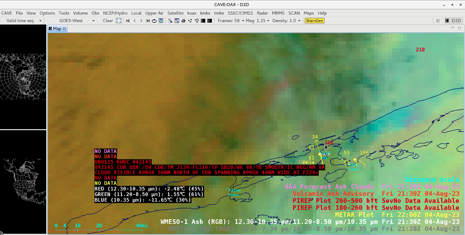
Pilot Report at 2139 UTC, mentioning volcanic ash (VA) visible 50 miles north of Cold Bay (CDB) at an altitude of 22000 ft [click to enlarge]
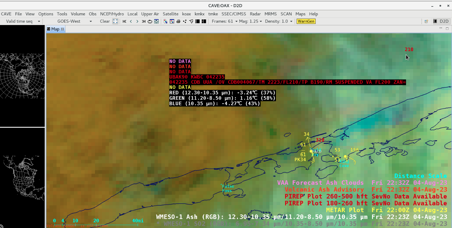
Pilot Report at 2223 UTC, describing volcanic ash (VA) suspended at an altitude of 20000 ft [click to enlarge]
View only this post
Read Less


