This website works best with a newer web browser such as Chrome, Firefox, Safari or Microsoft
Edge. Internet Explorer is not supported by this website.
SSEC Satellite Data Service is using McIDAS-X and HereGOES software packages to create imagery from the GOES-R Solar Ultra-Violet Imager (SUVI) instrument that monitors solar ultraviolet activity. Realtime SUVI images from both GOES-16 and GOES-18 can be viewed with the SSEC Geo... Read More
SUVI Fe171 imagery, 9 August 2023
SSEC Satellite Data Service is using McIDAS-X and HereGOES software packages to create imagery from the GOES-R Solar Ultra-Violet Imager (SUVI) instrument that monitors solar ultraviolet activity. Realtime SUVI images from both GOES-16 and GOES-18 can be viewed with the SSEC Geo Browser. Rick Kohrs at SSEC created the imagery in this blog post by loading images at different times, i.e., time-shifted by 2 hours. The animation above (three-dimensionality is achieved if the user crosses their eyes and focuses on the image that appears in the middle) shows data from the GOES-16 SUVI at 171 Å, from 1700-1900 UTC on 10 August 2023. A second animation, below, requires the use to don red/green glasses to perceive the three dimensions.
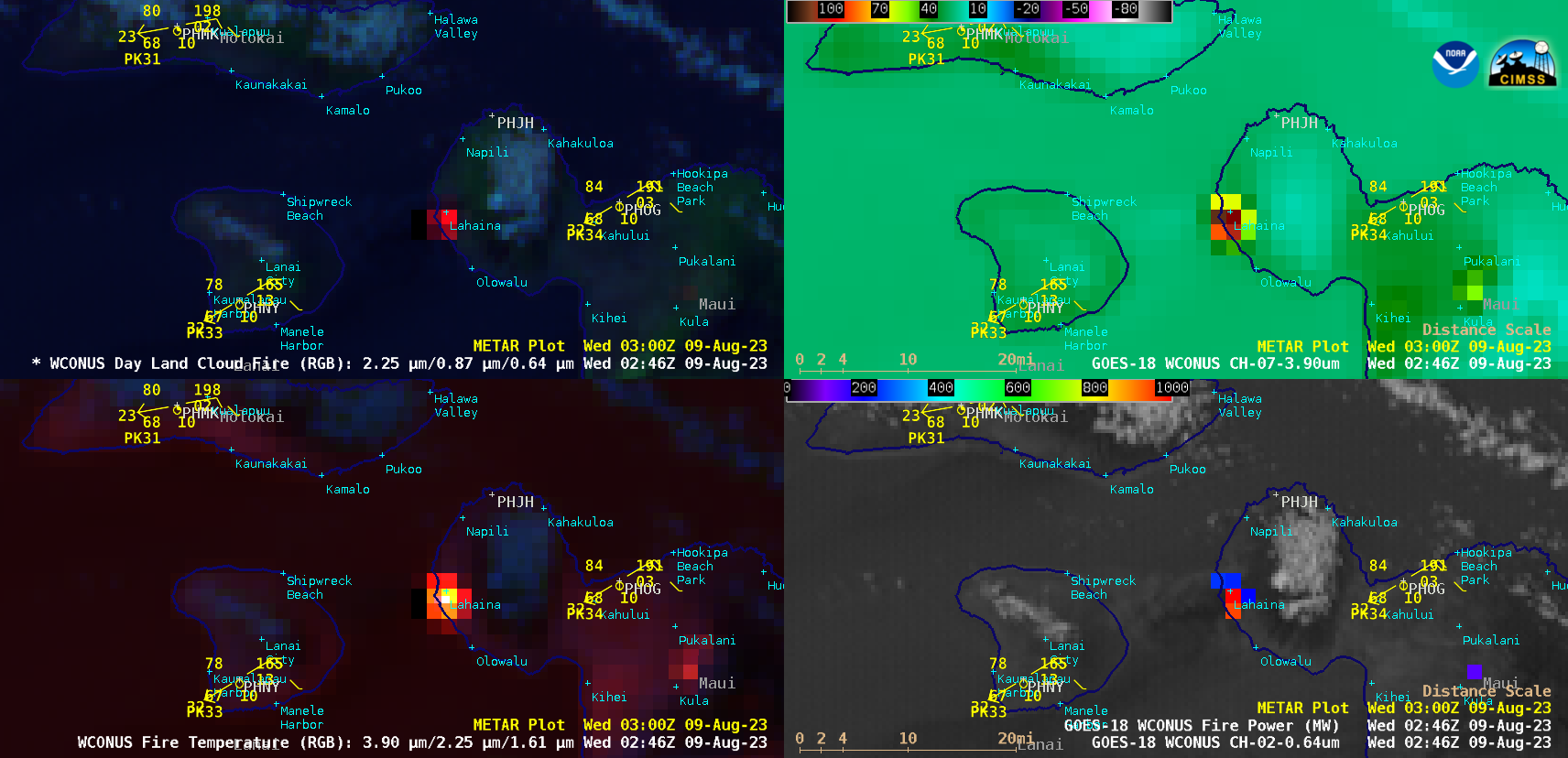
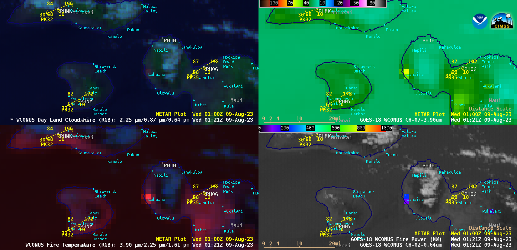
5-minute GOES-18 (GOES-West) images of Day Land Cloud Fire RGB, Shortwave Infrared (3.9 µm), Fire Temperature RGB and “Red” Visible (0.64 µm) with an overlay of Fire Power derived product (a component of the GOES Fire Detection and Characterization Algorithm FDCA) (above) showed thermal signatures associated with wildfires on the island of Maui in Hawai`i during the afternoon... Read More
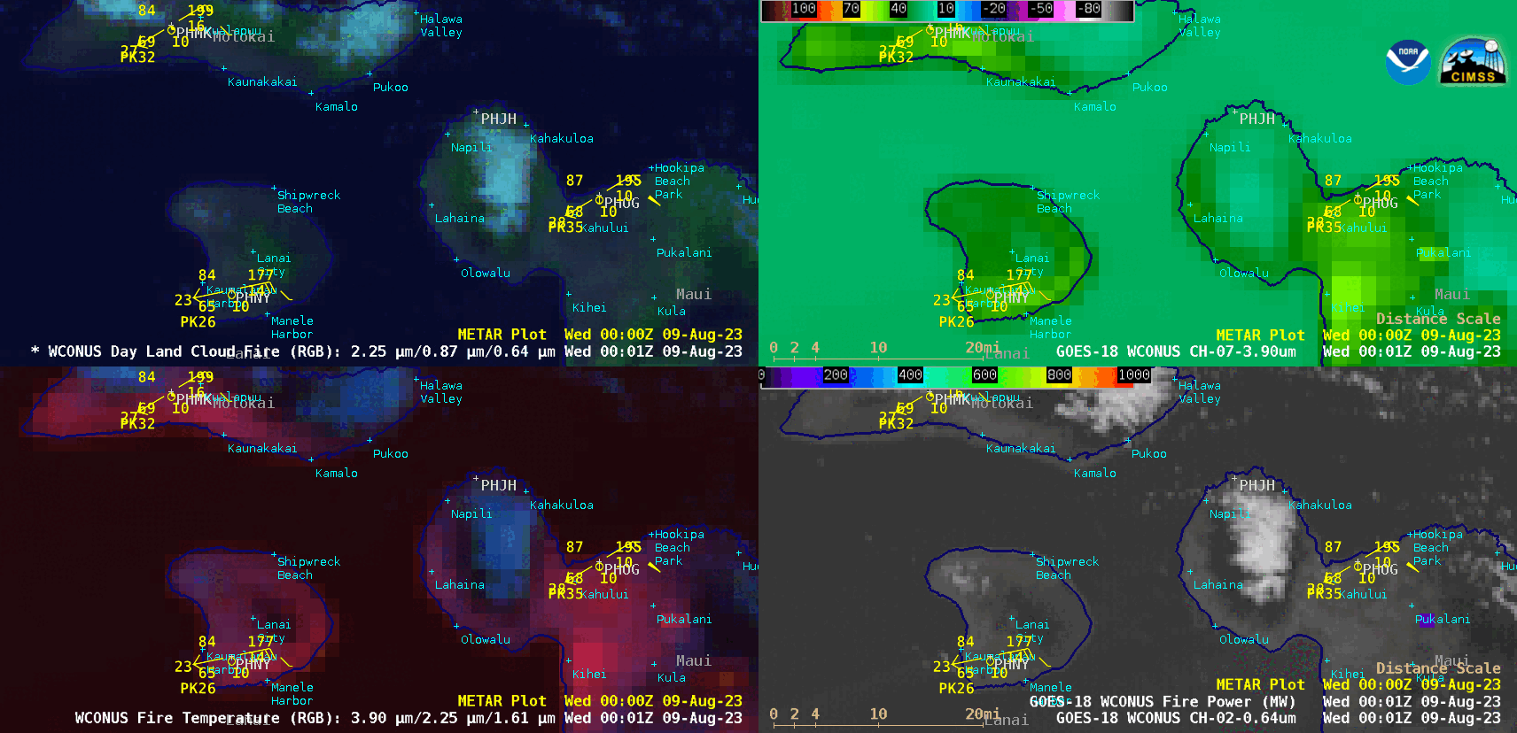
GOES-18 Day Land Cloud Fire RGB (top left), Shortwave Infrared (3.9 µm, top right), Fire Temperature RGB (bottom left) and “Red” Visible (0.64 µm) + Fire Power derived product (bottom right), from 0001-0901 UTC on 09 August [click to play animated GIF | MP4]
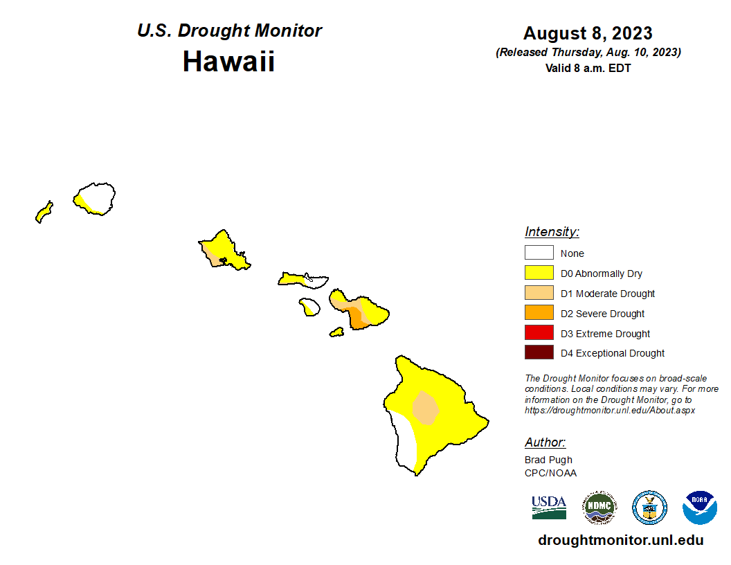
5-minute GOES-18 (GOES-West) images of Day Land Cloud Fire RGB, Shortwave Infrared (3.9 µm), Fire Temperature RGB and “Red” Visible (0.64 µm) with an overlay of Fire Power derived product (a component of the GOES Fire Detection and Characterization Algorithm FDCA)(above) showed thermal signatures associated with wildfires on the island of Maui in Hawai`i during the afternoon and evening hours (from 2:01 PM to 11:01 PM, local time) on 08 August 2023 — particularly near Lahaina (the West Maui Fire), where that large wildfire (which began to rapidly intensify around 0121 UTC on 09 August, or 3:21 PM local time on 08 August) caused extensive damage and forced evacuations, with at least 114 fatalities being reported. Near the center of the island, signatures of 2 other wildfires just northwest and northeast of Kula (the South Maui Fire and the Upcountry Fire, respectively) were also evident. Surface reports from nearby METAR sites showed that east-northeasterly wind gusts of 37-39 knots were occurring during that time period (however, a list of Local Storm Reports included wind gusts as high as 67 mph on Maui). The strong winds — along with dry vegetation from ongoing drought conditions across much of Maui County — contributed to the rapid intensification and spread of these wildfires. Additional aspects of the fire environment are discussed in this blog post.
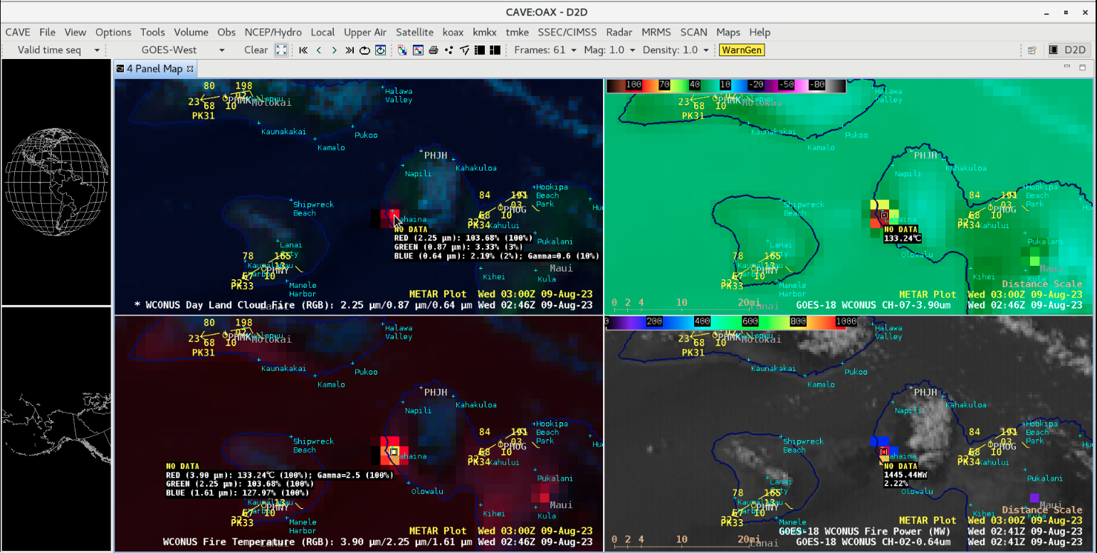
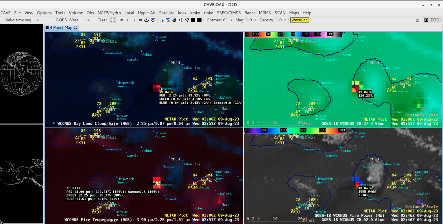
The West Maui Fire in the vicinity of Lahaina exhibited a maximum GOES-18 3.9 µm infrared brightness temperature of 133.24ºC at 0246 UTC (4:46 PM local time on 08 August), along with a maximum Fire Power value of 1885.04 MW (below).
Cursor-sampled GOES-18 Shortwave Infrared (3.9 µm) value of 133.24ºC at 0246 UTC, top right [click to enlarge]
Cursor-sampled GOES-18 Fire Power value of 1885.24 MW at 0246 UTC, bottom right [click to enlarge]
A closer look at GOES-18 Shortwave Infrared images over a longer period of time — from 0001 UTC on 08 August to 0601 UTC on 10 August (below) — revealed that the first of the 3 large Maui wildfires was the Upcountry Fire, whose thermal signature began to rapidly intensify SE of Pukalani around 1101 UTC on 08 August (1:01 AM local time); several hours later, the West Maui Fire thermal signature then began to rapidly intensify near Lahaina around 0121 UTC on 09 August (3:21 PM local time on 08 August), followed by the South Maui Fire whose thermal signature began to rapidly intensify NW of Kula around 0401 UTC on 09 August (6:01 PM local time on 08 August). The GOES-18 thermal signatures of all 3 of these large Maui wildfires had generally diminished by about 0601 UTC on 10 August (8:01 PM local time on 09 August) — although the fires were still not 100% contained at that point.
GOES-18 Shortwave Infrared (3.9 µm) images, from 0001 UTC on 08 August to 0601 UTC on 10 August [click to play animated GIF | MP4]
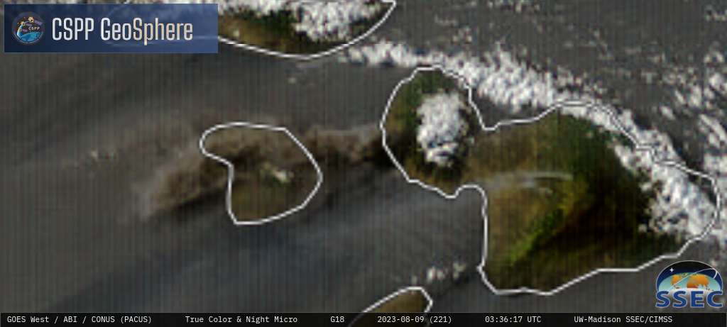
GOES-18 True Color RGB images (centered on Lahaina) from the CSPP GeoSphere site (below) showed the large and very dense smoke plume from the Lahaina wildfire as it streamed westward across the island of Lanai — along with 2 more narrow smoke plumes from the smaller fires near the center of Maui.
GOES-18 True Color RGB images [click to play MP4 animation]
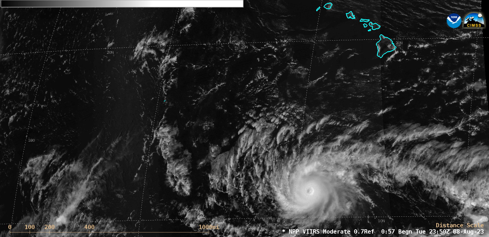
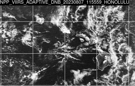
Suomi-NPP VIIRS Day/Night Band (0.7 µm) image valid at 0036 UTC on 09 August [click to enlarge]
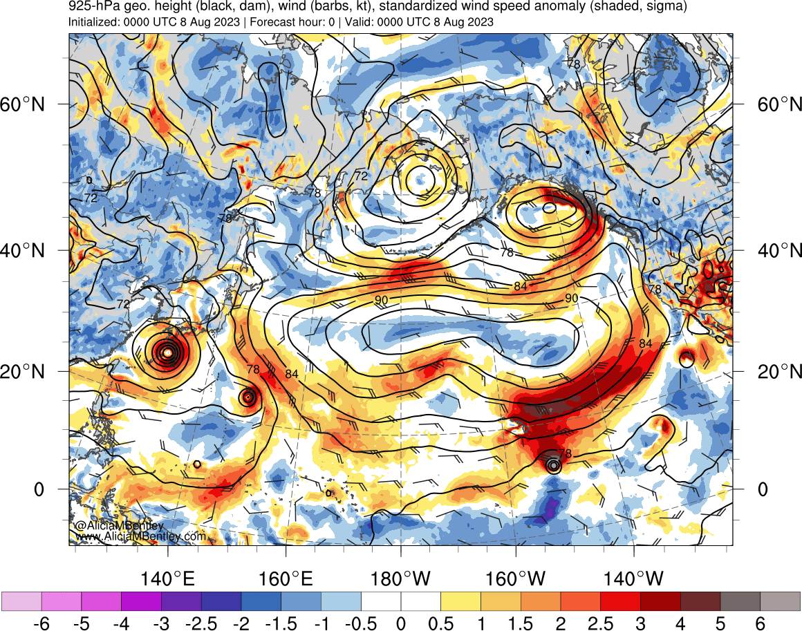
A Suomi-NPP VIIRS Day/Night Band (0.7 µm) image valid at 0036 UTC on 09 August (above) showed that compact Category 4 Hurricane Dora was centered about 800 miles south-southwest of Hawai`i. The arrival of a burst of easterly/northeasterly trade winds across the island chain — partially accelerated by the pressure gradient between a strong anticyclone to the north and Hurricane Dora to the south (for more details, see this Climate Connections summary) — brought a period of anomalously strong lower-tropospheric wind speeds (source), shown below in shades of red to gray (Maui is centered near 21º N latitude, 156º W longitude).
925 hPa wind speed anomaly, 0000 UTC on 08 August to 1200 UTC on 09 August [click to enlarge]
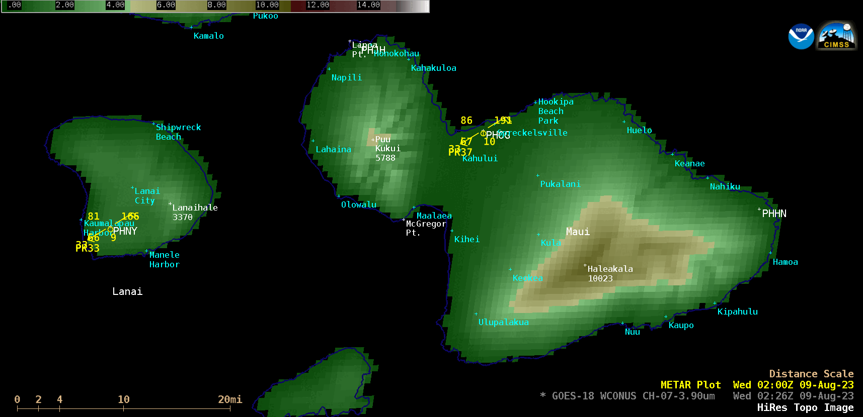
A downslope enhancement (from the 5788-foot summit of Pu`u Kukui) likely played an additional role in creating stronger winds in the vicinity of the Lahaina wildfire — as well as in the area of the 2 wildfires near Kula, with downslope flow from the 10023-foot summit of Haleakala (below).
GOES-18 Shortwave Infrared (3.9 µm) and topography [click to enlarge]
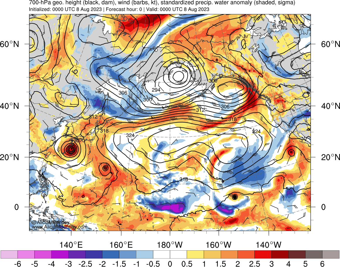
Accompanying the easterly trade wind burst was the arrival of anomalously low Total Precipitable Water (shades of blue), depicted below.
700 hPa height/wind and Total Precipitable Water anomaly, 0000 UTC on 08 August to 1200 UTC on 09 August [click to enlarge]
A 2-day animation of GOES-18 Mid-level Water Vapor (6.9 µm) images from 0001 UTC on 08 August to 0201 UTC on 10 August (below) showed 2 areas exhibiting warm 6.9 µm infrared brightness temperatures (darker shades of orange) — indicative of dry air within the middle troposphere — passing over parts of Hawai`i during that time period.
GOES-18 Mid-level Water Vapor (6.9 µm) images, from 0001 UTC on 08 August to 0201 UTC on 10 August [click to play animated GIF | MP4]
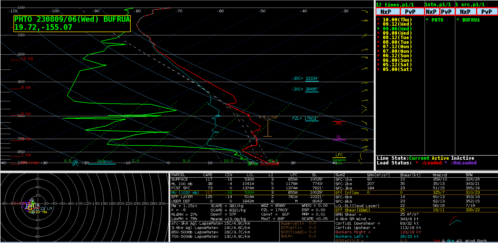
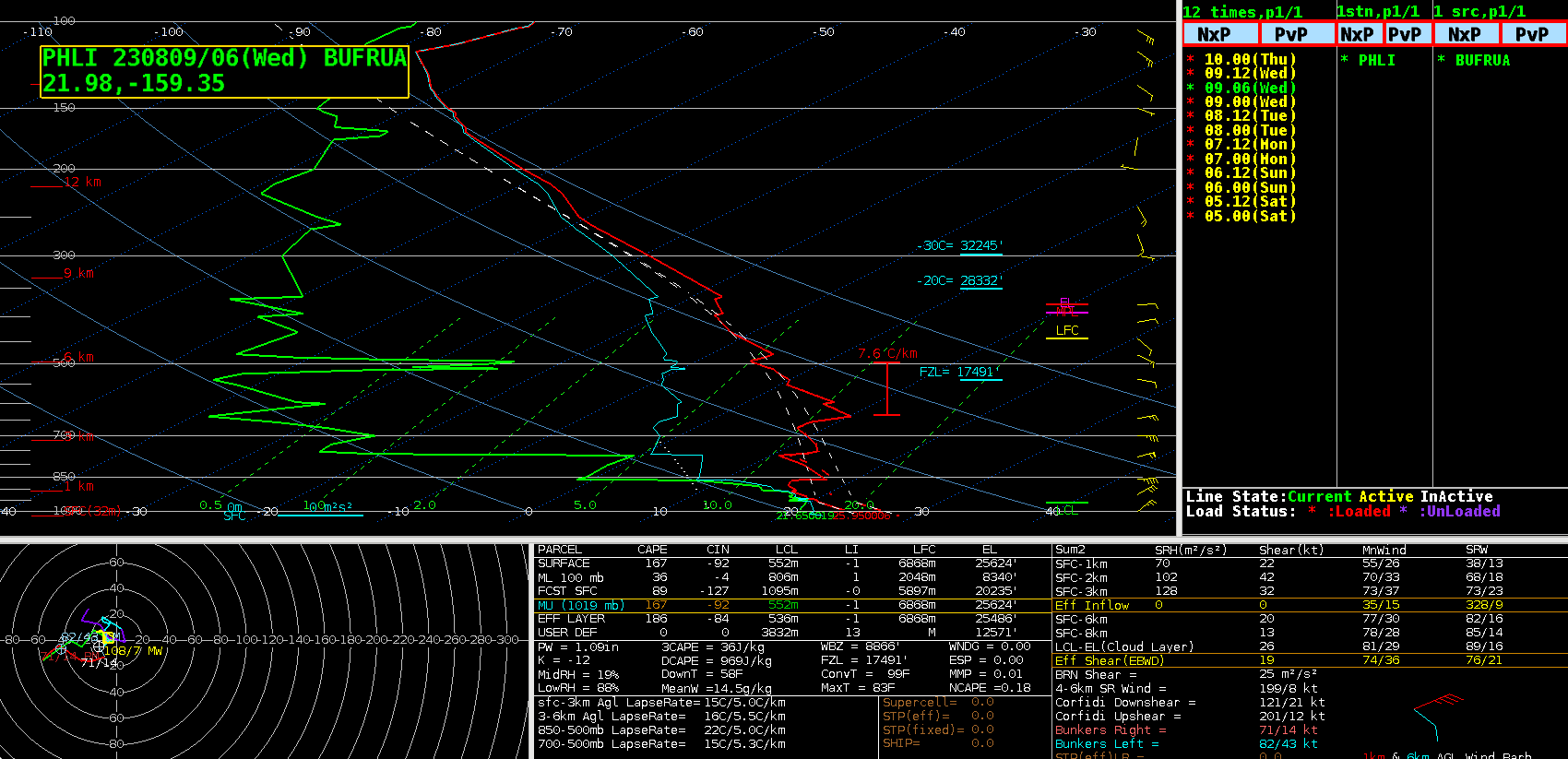
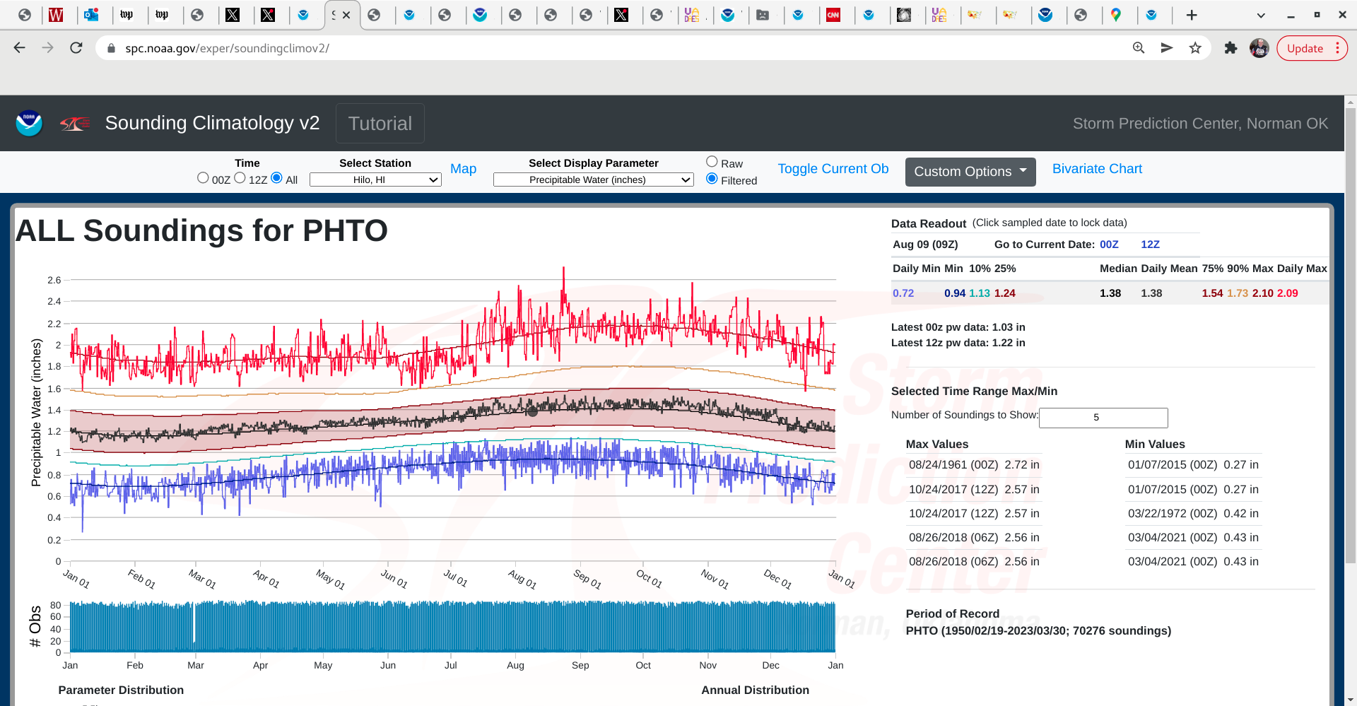
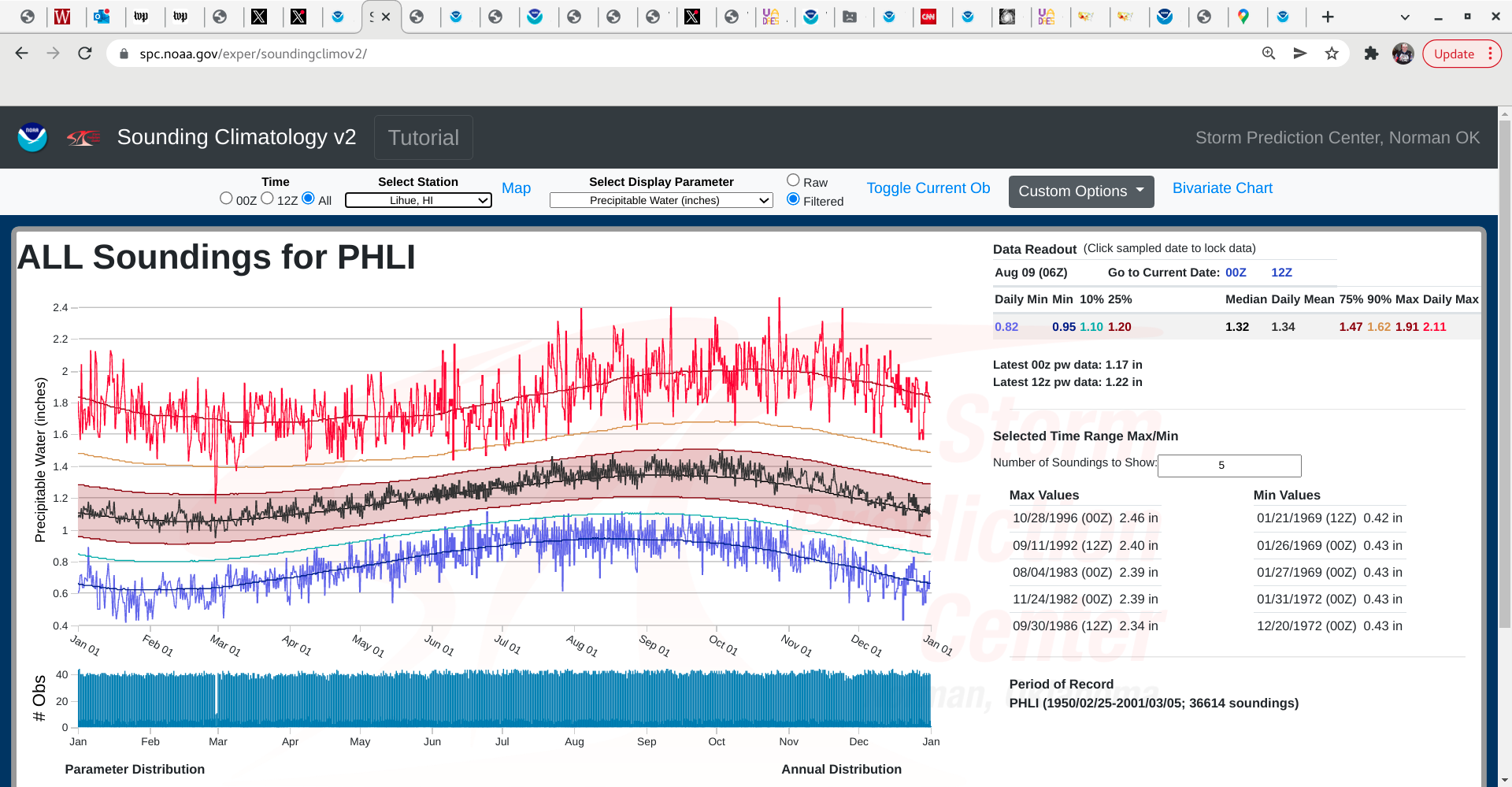
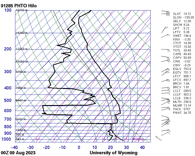
Plots of rawinsonde data from Hilo and Lihue at 0600 UTC on 09 August (below) showed the presence of very dry air above the trade wind inversion at that time — and a nearly dry adiabatic lapse rate existed from below the base of the inversion (located at an altitude around 5600 ft at Hilo, and 4100 ft at Lihue) to the surface, which would have aided the downward transport of that dry air aloft (enhancing the already-dangerous wildfire environment at the surface). Total Precipitable Water values were 1.15 inches at Hilo (compared to the daily mean value of 1.38 inches) and 1.09 inches at Lihue (compared to the daily mean value of 1.34 inches).
Plot of rawinsonde data from Hilo at 0600 UTC on 09 August [click to enlarge]
Plot of rawinsonde data\ from Lihue at 0600 UTC on 09 August [click to enlarge]
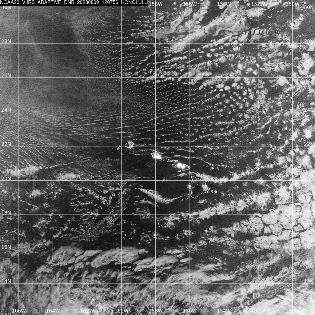
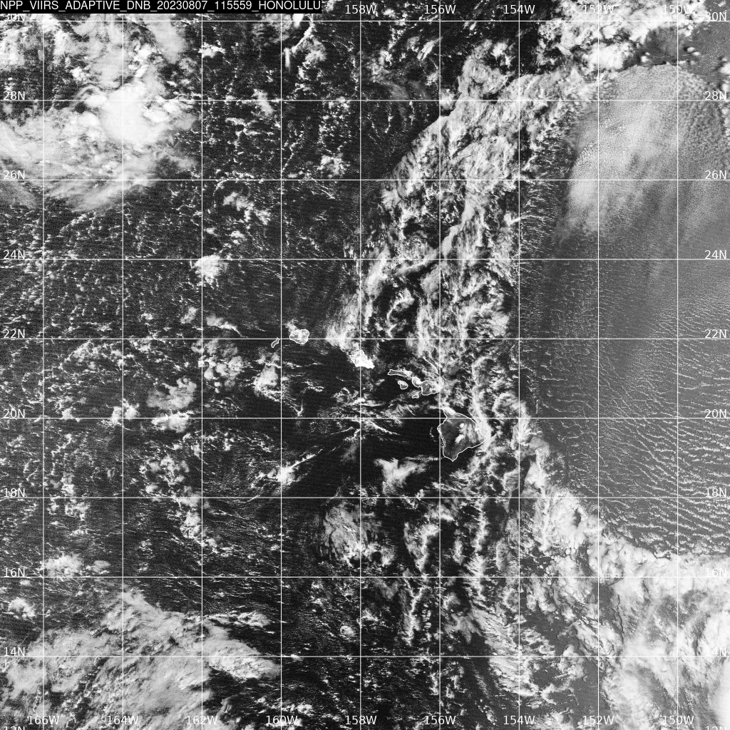
Day Night Band imagery from Suomi NPP (on 7 August) and NOAA-20 (on 9 August) shows the increase in emitted light over western Maui as the fires burned. (Imagery downloaded from the HCC direct broadcast site in Honolulu and cropped. The full-sized toggle is here).
Day NIght Band VIIRS visible (0.7 µm) imagery, ca. 1200 UTC on 7 and 9 August 2023 (courtesy Scott Lindstrom, CIMSS)
VIIRS Day Night Band captured the glow of the deadly wind-whipped flames burning on Maui during the predawn hours of August 9th. We have more imagery and information on the destructive event at https://t.co/20TBEzGMwqpic.twitter.com/HDDh8iu6Bt
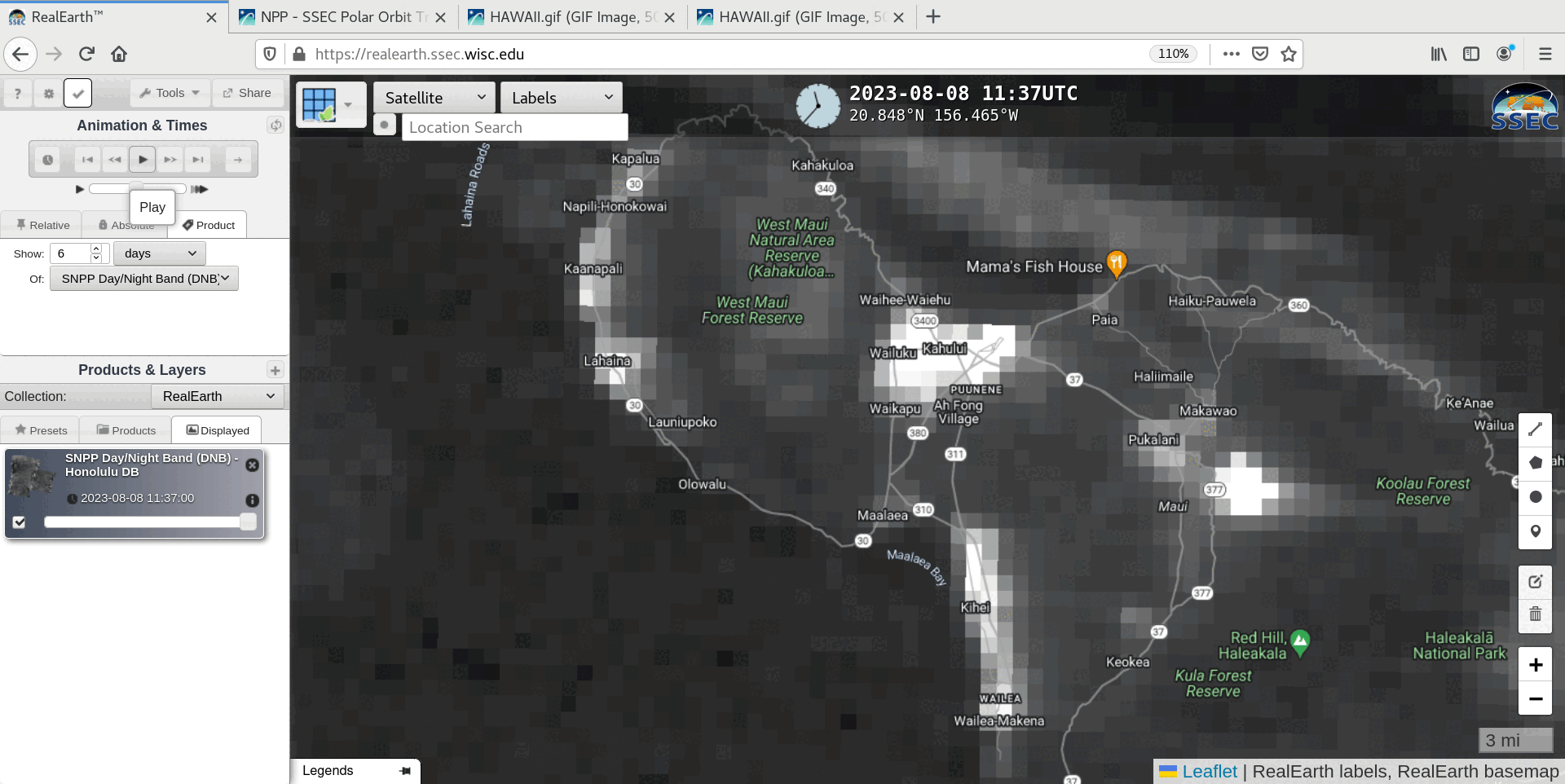
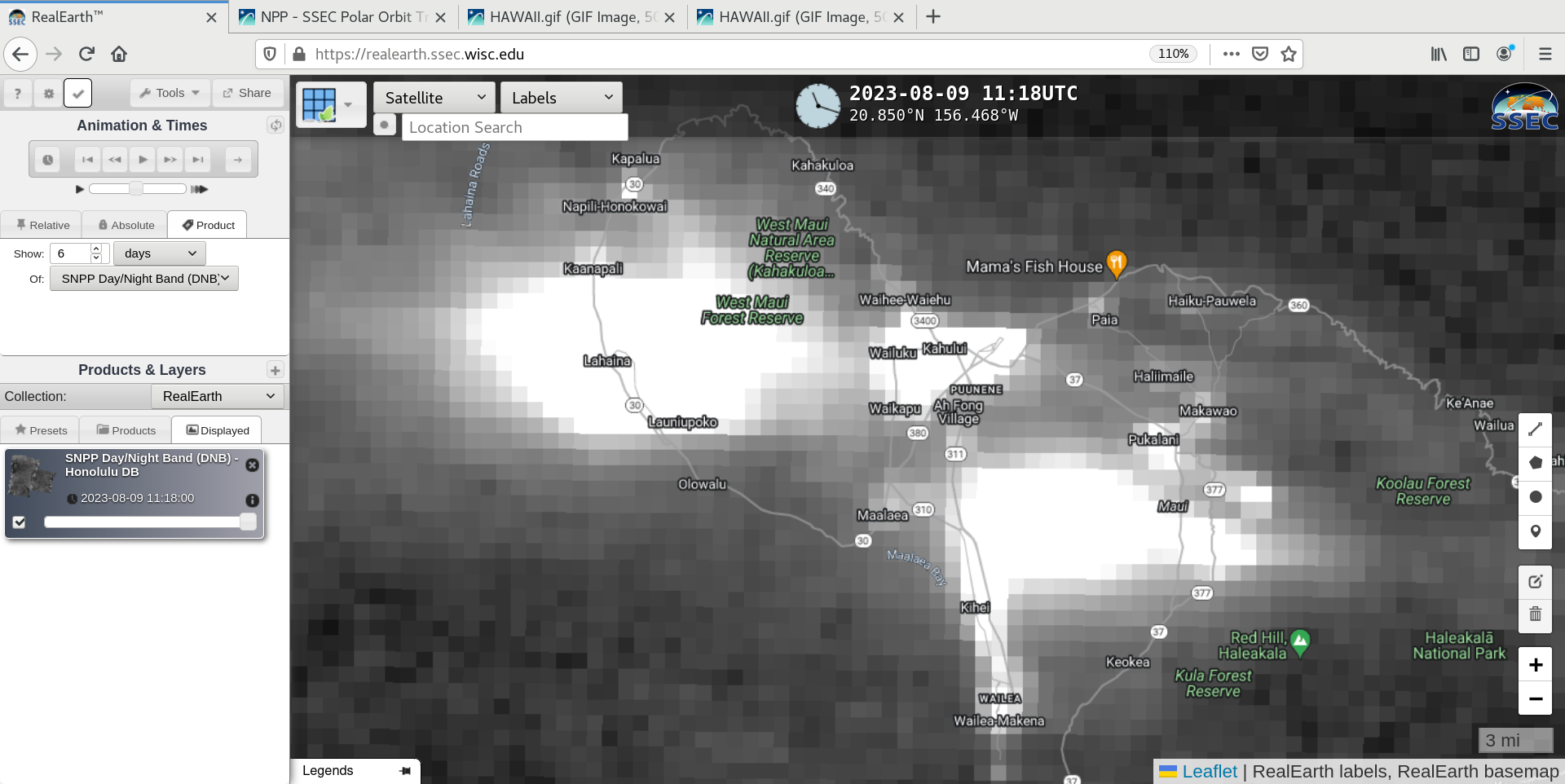
In a sequence of Suomi-NPP VIIRS Day/Night Band (0.7 µm) images from before (08 August), during (09 August) and after (11 August) the Maui wildfires, viewed using RealEarth(below), the intense glow of the West Maui and South Maui/Upcountry Fires was quite prominent in the 09 August image — and a reduction in the intensity of city light emission (due to fire-related power outages) was evident across the Lahaina and West Maui areas in the 11 August image.
Suomi-NPP VIIRS Day/Night Band (0.7 µm) images before (08 August), during (09 August) and after (11 August) the Maui wildfires [click to enlarge]
Additional aspects of the Maui Fires were discussed in this Satellite Book Club presentation.
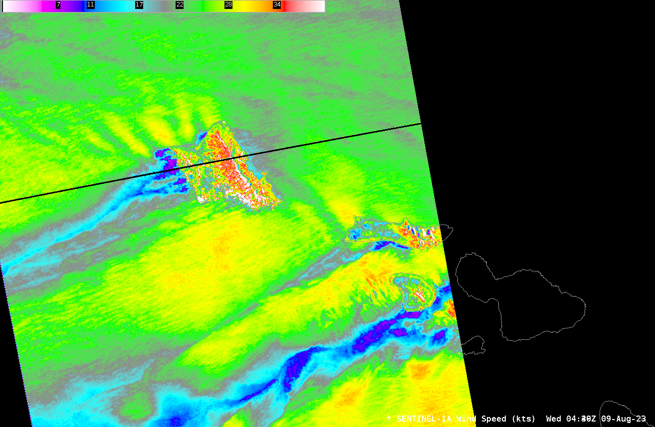
Deadly fires on the island of Maui occurred in an environment favorable to fire development: dry and windy. What kind of satellite data could be used to assess those conditions? Sentinel-1A overflew the western Hawai’ian islands near sunset on 8 August 2023 (that is, at 0440 UTC on 9 August), as shown above. Widespread 30-knot winds... Read More
Sentinel-1A SAR Winds, 0439-0440 UTC on 9 August 2023
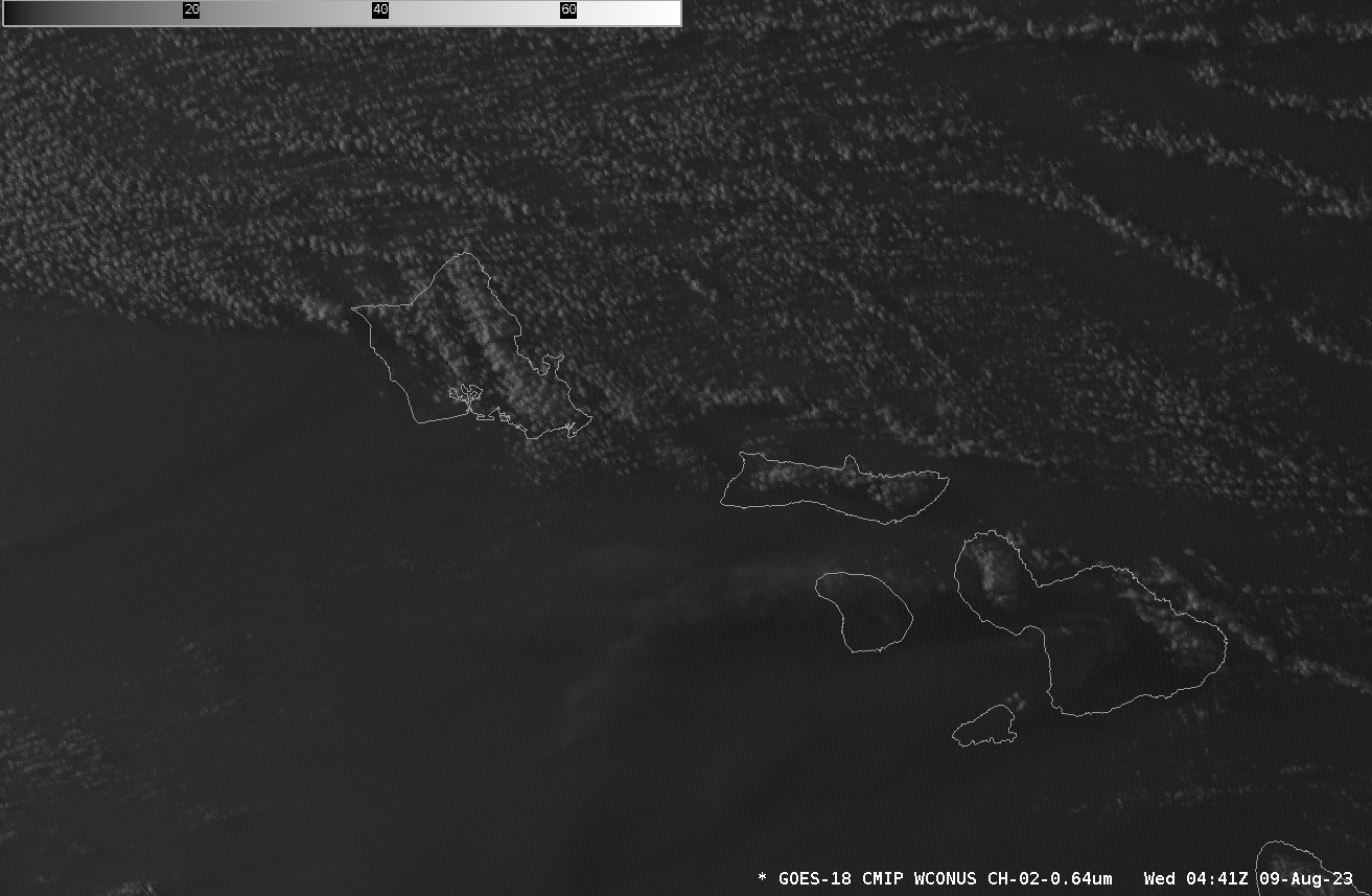
Deadly fires on the island of Maui occurred in an environment favorable to fire development: dry and windy. What kind of satellite data could be used to assess those conditions? Sentinel-1A overflew the western Hawai’ian islands near sunset on 8 August 2023 (that is, at 0440 UTC on 9 August), as shown above. Widespread 30-knot winds (yellow in the enhancement used) are indicated. The island of Maui was just missed by this scan. The SAR Winds are shown below in a toggle with GOES-18 Visible imagery. A smoke plume that extends west of Maui is faintly apparent. Low clouds are present east and north of the Hawai’ian islands, but are absent to the south and west. The motion of these low clouds can be tracked to infer winds.
GOES-18 Visible Imagery (Band 2, 0.64 µm), brightened, toggling with SAR Winds, 0441 UTC on 9 August 2023 (Click to enlarge)
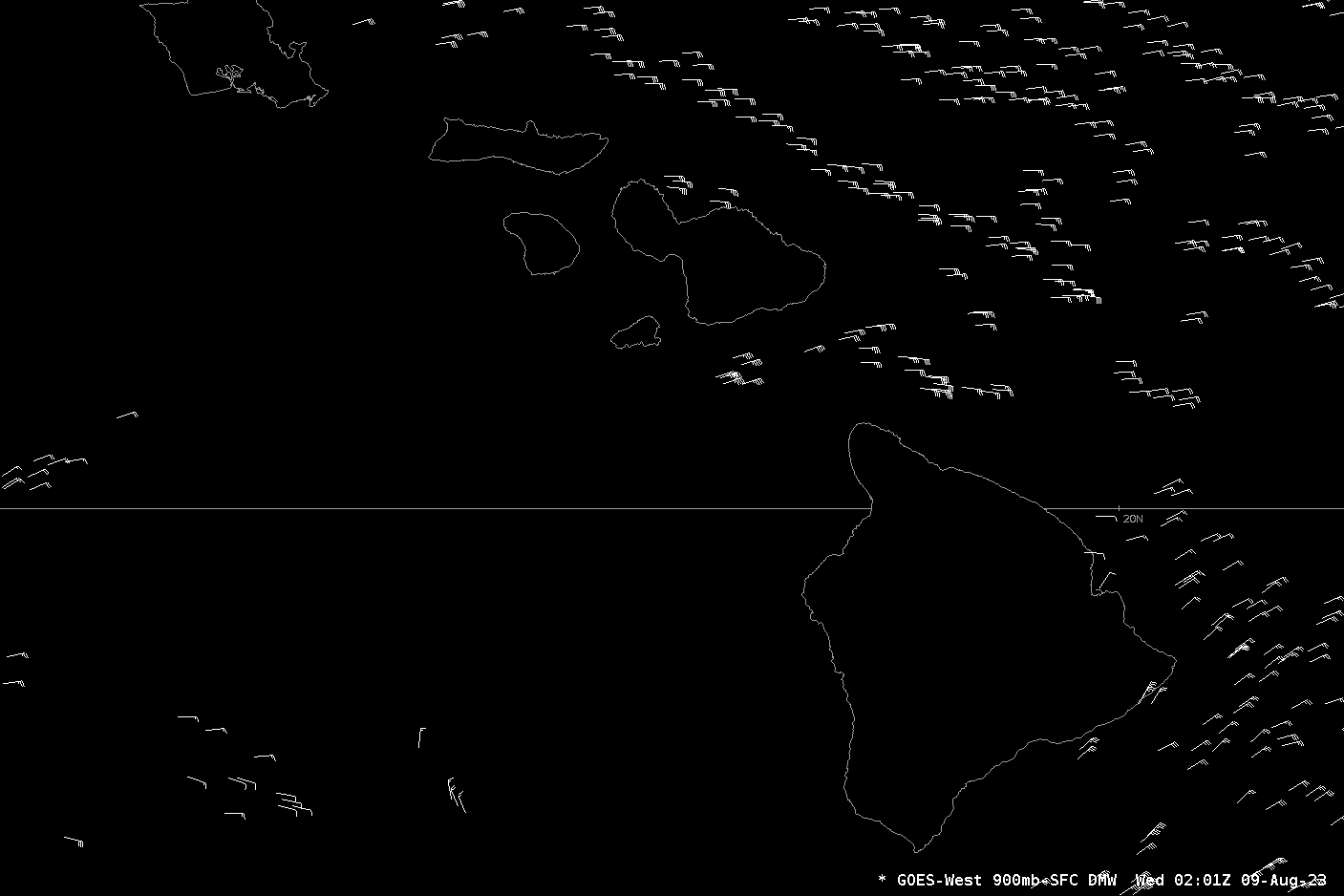
GOES-18 Derived Motion Wind vectors, shown below, hourly from 0201-0701 on 9 August, show widespread values of 30-35 knots to the east and north of the Hawai’ian island chain. The features tracked to infer the winds were from near-surface to 900 mb.
GOES-18 Derived Motion Wind vectors, 0201-0701 UTC on 9 August 2023 (Click to enlarge)
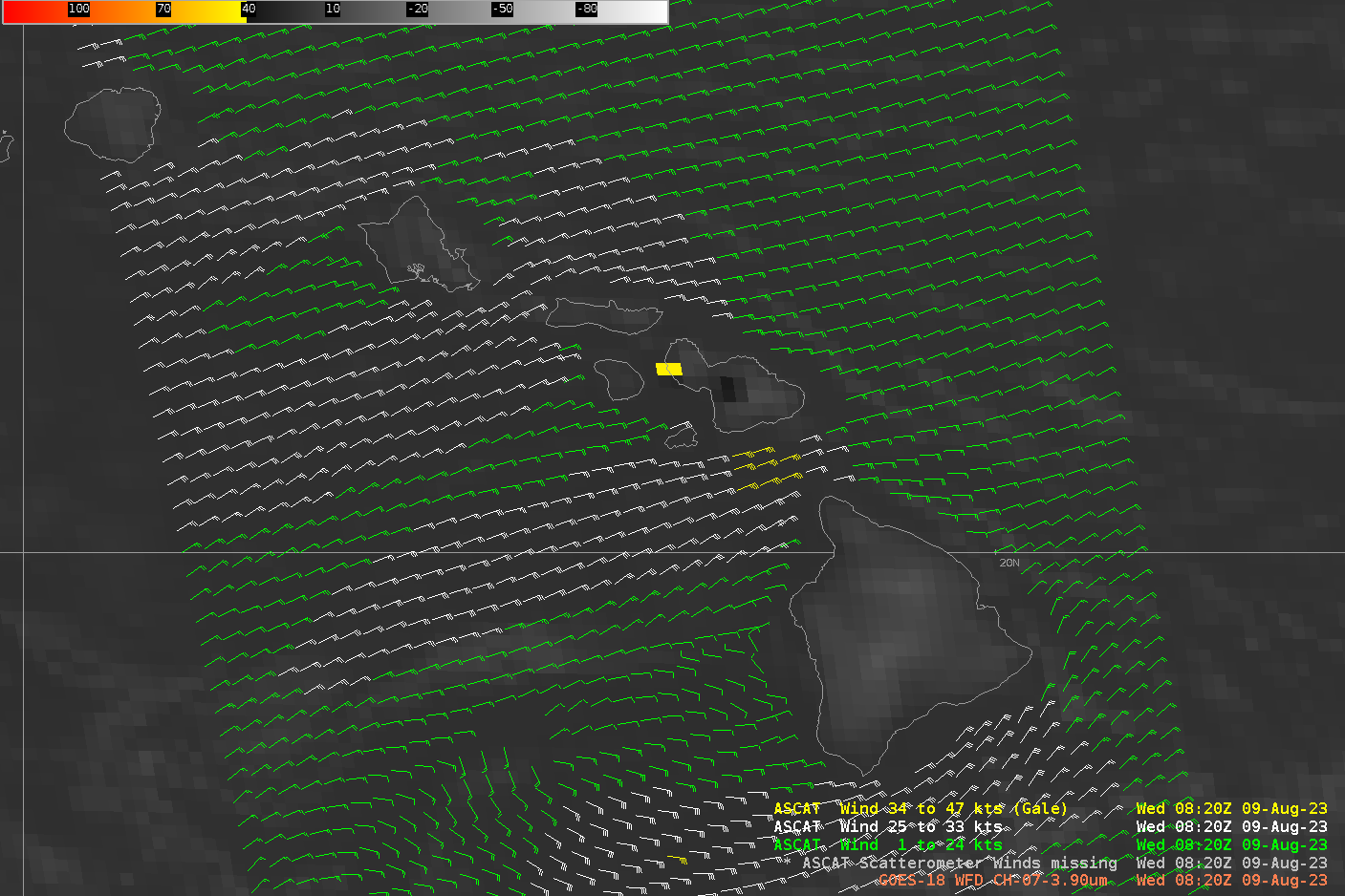
Metop-C overflew the Hawai’ian islands shortly after 0800 UTC on 9 August, and Advanced Scatterometer (ASCAT) winds from that pass are shown below, overlain on top of GOES-18 Band 7 (Shortwave Infrared, 3.9 µm) imagery that shows the signatures of the two fires (yellow and black) on Maui. Winds of 25-30 knots are widespread near the Hawai’ian islands, with somewhat weaker winds to the north and east. Stronger winds — gales — are detected in the Alenuihaha channel between Hawai’i and Maui.
GOES-18 Shortwave Infrared Imagery (Band 7, 3.9 µm), , toggling and Metop-C ASCAT Winds, 0820 UTC on 9 August 2023 (Click to enlarge)
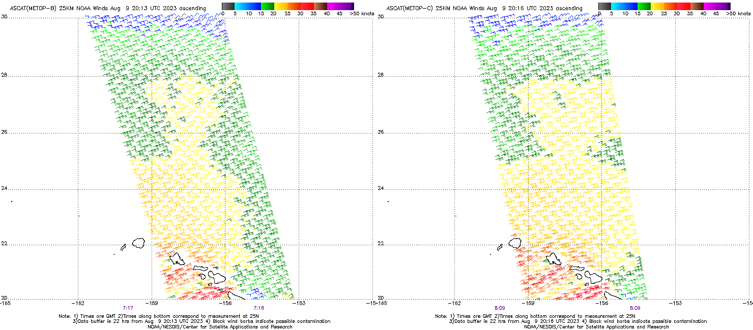
Metop-B also sampled this region, but a bit earlier than Metop-C. Wind plots for both satellites (taken from this site) are shown below. Winds are strongest surrounding the Hawai’ian island chain.
Metop-B ASCAT Winds (left, 0717 UTC) and Metop-C ASCAT Winds (right, 0809 UTC) on 9 August 2023 (Click to enlarge)
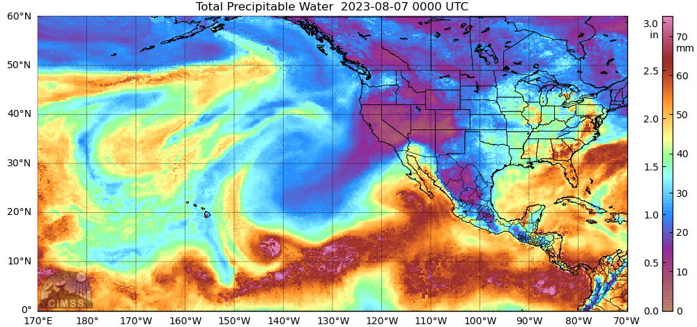
Three different wind data sources above highlight the strong environmental winds surrounding the Hawai’ian island chain. How dry was the environment? The MIMIC Total Precipitable Water animation below, shows significant drying occurring between 0000 UTC 7 August and 0000 UTC 9 August as the moisture associated with Hurricane Dora moves south of the islands.
MIMIC Total Precipitable Water estimates, 0000 UTC 7 August – 0000 UTC 9 August 2023 (Click to enlarge)
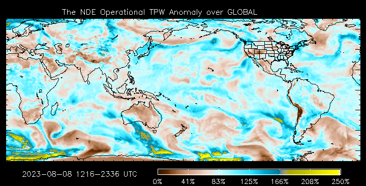
The percent-of-normal TPW values surrounding Hawai’i (source) around 0000 UTC on 9 August,shown below, were 40-50%.
Percent-of-Normal TPW, ca. 0000 UTC on 9 August 2023 (Click to enlarge)
The 0000 UTC Sounding from Hilo (here, from this source), shows a computed TPW of 1.36″. This SPC site shows that value to be dryer than normal.
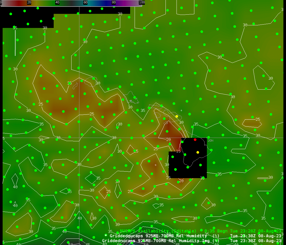
NOAA-20 NUCAPS data can be used to assess moisture at various levels. NOAA-20 overflies Hawai’i at around 0000 and 1200 UTC daily, and the toggle below shows gridded NUCAPS estimates of relative humidity in the 925-700 mb layer at 2338 UTC on 8 August and 1205 UTC on 9 August. Sounding availability points are also shown, and the NUCAPS retrievals were converging (green points) over most of the domain shown.
Gridded NUCAPS estimates of Relative Humidity in the 925-700 mb layer, 2338 UTC/08 August and 1205 UTC/09 August 2023 (Click to enlarge)
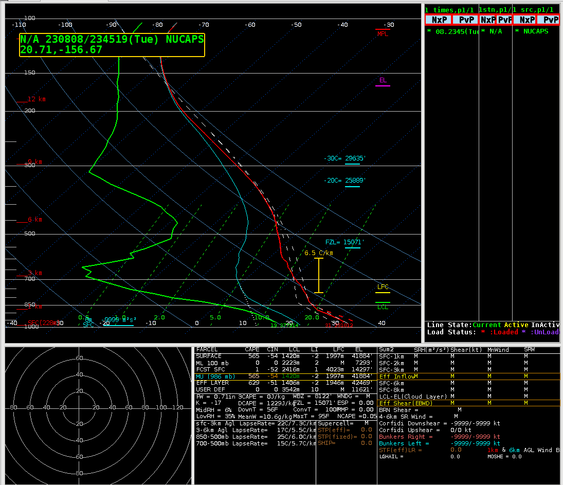
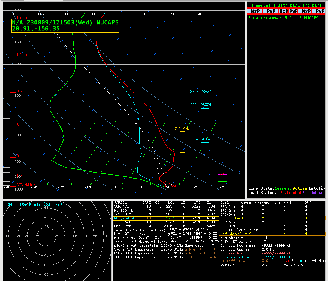
At 2338 UTC on 08 August, a successful retrieval is indicated just west of Maui; at 1205 UTC on 09 August, a successful retrieval is apparent near the northern shore of Maui. The two NUCAPS soundings at those points are shown below.
NUCAPS Sounding, 2345 UTC on 8 August 2023, Lat/Lon as indicated, just west of Maui (Click to enlarge)NUCAPS Sounding, 1215 UTC on 9 August 2023, Lat/Lon as indicated, near the north shore of Maui (Click to enlarge)
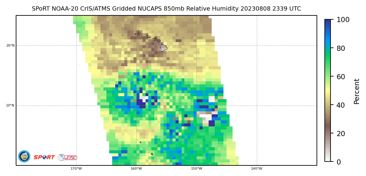
Gridded NUCAPS data are also available online for Hawaii at this website. The animation below toggles through relative humidity estimates at 850, 700, 500 and 300 mb. Dry air is indicated.
Relative Humidity at 850, 700, 500 and 300 mb, 2339 UTC on 8 August 2023 (click to enlarge)
Many satellite products can help a forecaster understand the environment when dangerous weather is expected. This snippet from a Forecast Discussion from late on 3 August shows that Fire Weather was anticipated to occur over the Hawai’ian Islands long before the fires occurred.
GOES-18 (GOES-West) Day Land Cloud Fire RGB, Shortwave Infrared (3.9 µm), “Clean” Infrared Window (10.3 µm) and “Red” Visible (0.64 µm) images with an overlay of the Fire Power derived product — Fire Power is a component of the GOES Fire Detection and Characterization Algorithm FDCA — (above) showed signatures associated with a wildfire (located about 20 miles WNW of Mayo,... Read More
GOES-18 Day Land Cloud Fire RGB (top left), Shortwave Infrared (3.9 µm, top right), “Clean” Infrared Window (10.3 µm) (bottom left) and “Red” Visible (0.64 µm) + Fire Power derived product (bottom right) [click to play animated GIF | MP4]
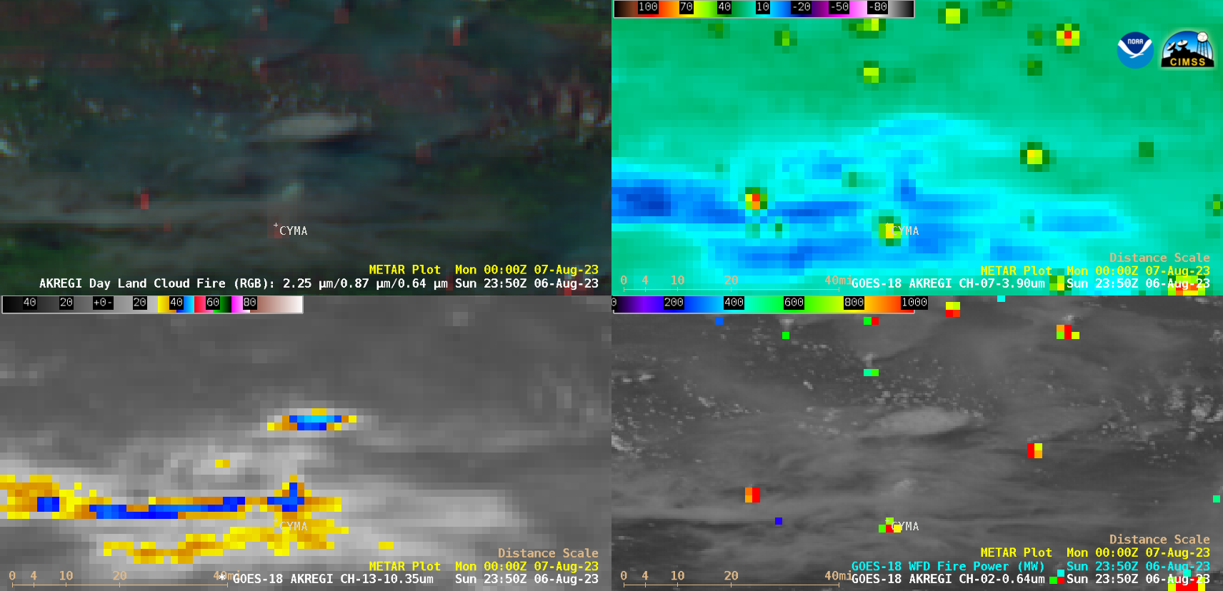
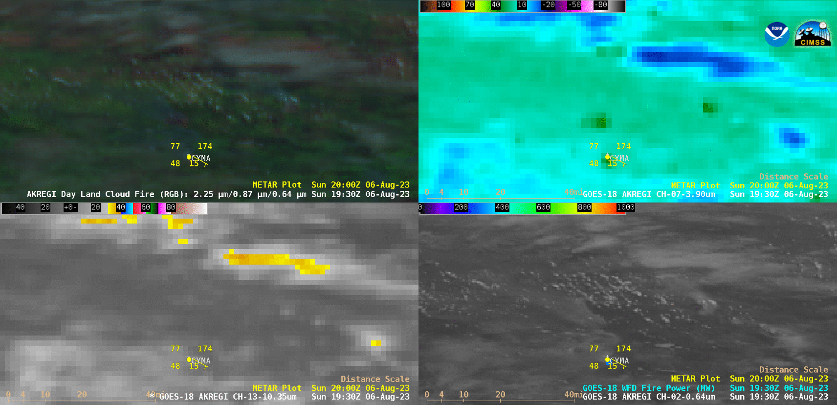
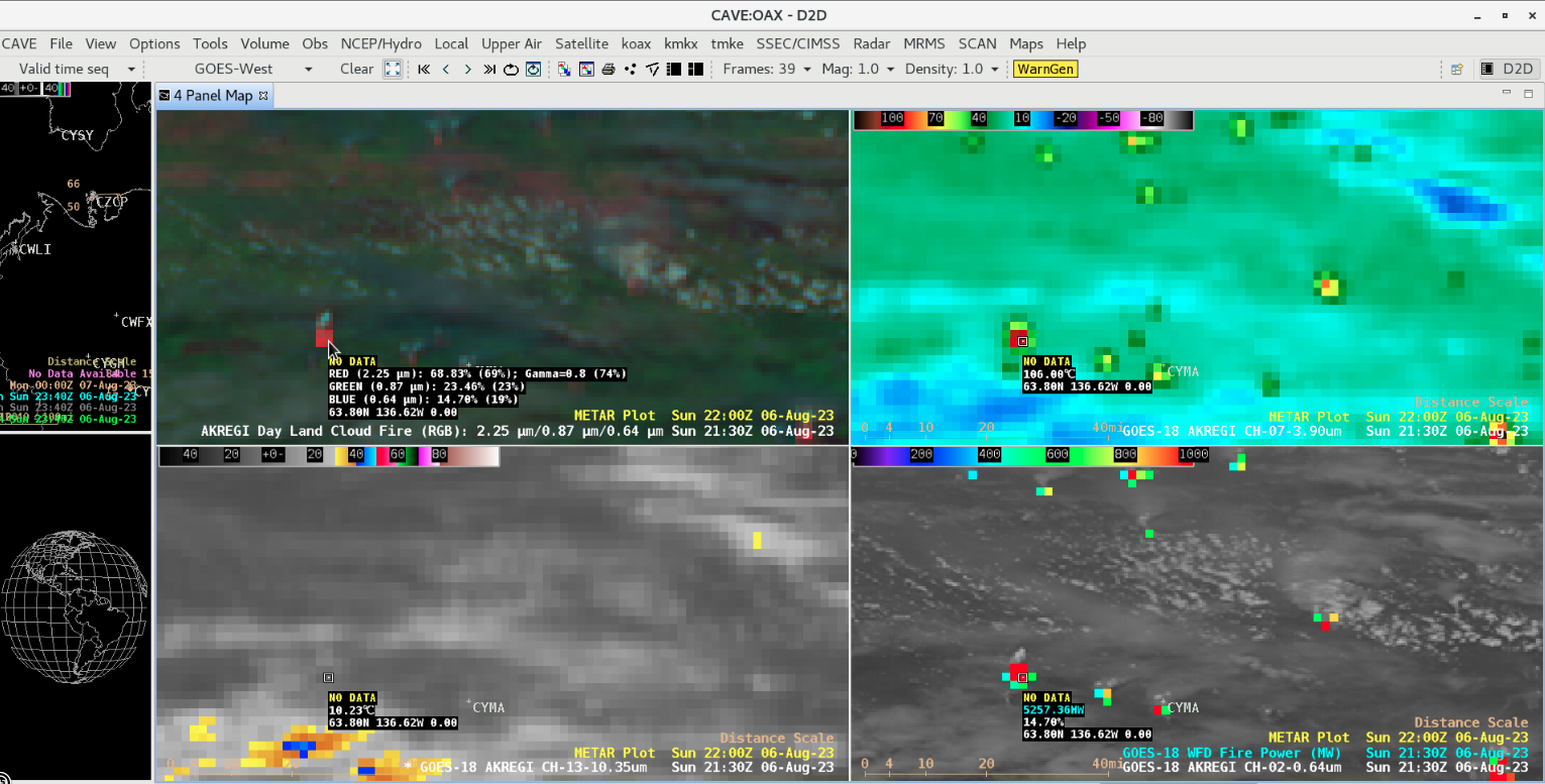
GOES-18 (GOES-West)Day Land Cloud Fire RGB, Shortwave Infrared (3.9 µm), “Clean” Infrared Window (10.3 µm) and “Red” Visible (0.64 µm) images with an overlay of the Fire Power derived product — Fire Power is a component of the GOES Fire Detection and Characterization Algorithm FDCA — (above) showed signatures associated with a wildfire (located about 20 miles WNW of Mayo, Yukon CYMA) that produced a pyrocumulonimbus (pyroCb) cloud late in the day on 06 August 2023.
At 2130 UTC, the wildfire exhibited a maximum 3.9 µm infrared brightness temperature of 106C, with a Fire Power value of 5257 MW (below).
Cursor-sampled values of GOES-18 Day Land Cloud Fire RGB (top left), Shortwave Infrared (3.9 µm, top right), “Clean” Infrared Window (10.3 µm) (bottom left) and “Red” Visible (0.64 µm) + Fire Power derived product (bottom right) at 2130 UTC [click to enlarge]
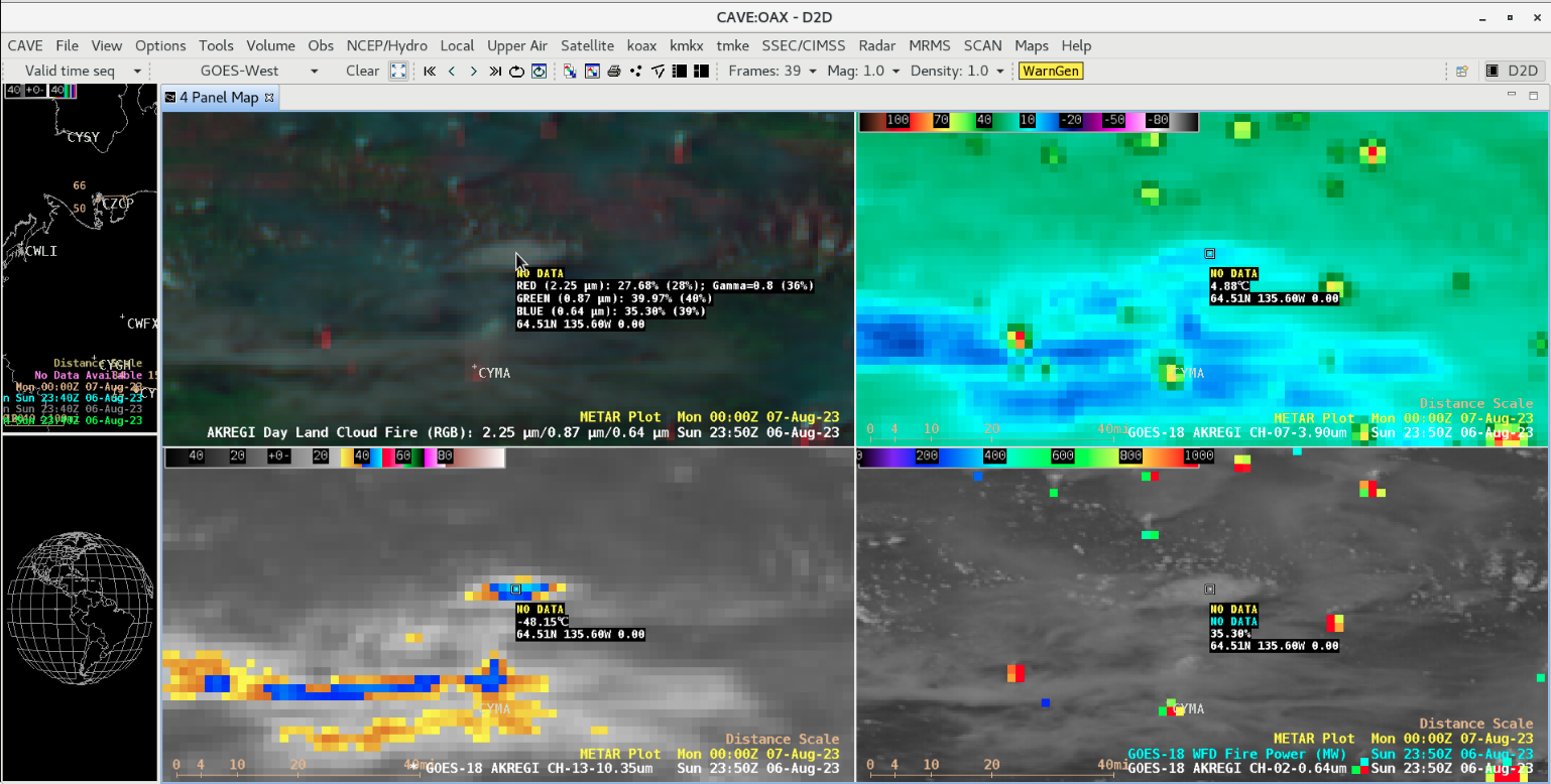
The pyroCb cloud exhibited a cloud-top 10.3 µm infrared brightness temperature as cold as -48.15C at 2350 UTC (below).
Cursor-sampled values of GOES-18 Day Land Cloud Fire RGB (top left), Shortwave Infrared (3.9 µm, top right), “Clean” Infrared Window (10.3 µm) (bottom left) and “Red” Visible (0.64 µm) + Fire Power derived product (bottom right) at 2350 UTC [click to enlarge]


