GOES-16 (GOES-East) True Color RGB images created using Geo2Grid (above) showed the south-southeastward drift of an ash-laden volcanic cloud from Cumbre Vieja on La Palma in the Canary Islands on 09 October 2021. Since this most recent ongoing eruptive period began on 19 September, intermittent periods of volcanic clouds with an elevated ash content... Read More
GOES-16 True Color RGB images [click to play animation | MP4]
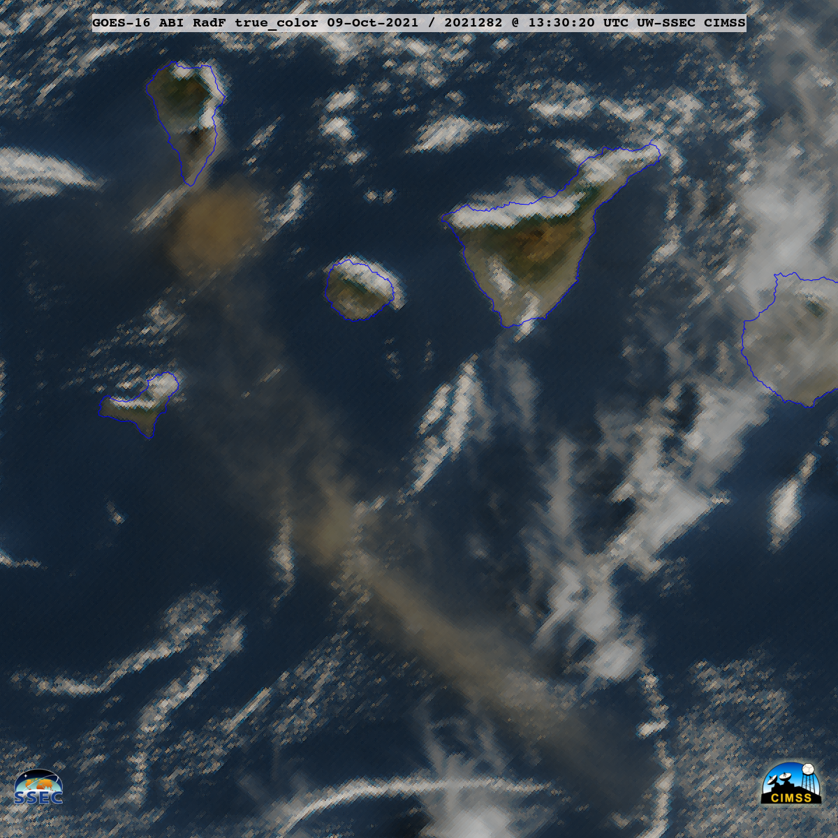
GOES-16 (GOES-East) True Color RGB images created using Geo2Grid (above) showed the south-southeastward drift of an ash-laden volcanic cloud from Cumbre Vieja on La Palma in the Canary Islands on 09 October 2021. Since this most recent ongoing eruptive period began on 19 September, intermittent periods of volcanic clouds with an elevated ash content have been observed — and on this day, the darker tan to light brown appearance was an indication that higher ash concentrations were likely.
In the corresponding GOES-16 Ash RGB images (below), increasing shades of pink — which suggest a higher ash content — became apparent within a semi-circular volcanic cloud element after 1100 UTC.
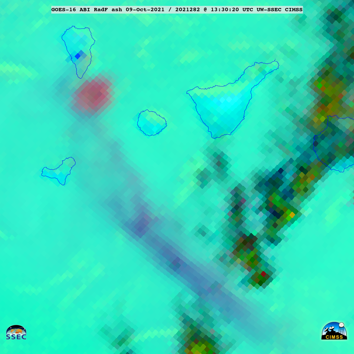
GOES-16 Ash RGB images [click to play animation | MP4]
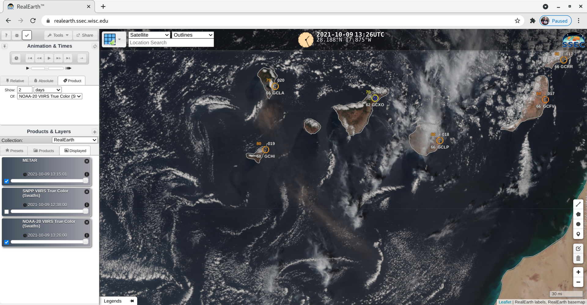
A NOAA-20 VIIRS True Color image as viewed using RealEarth (below) also showed the darker tan to light brown shades of the ash-laden volcanic cloud.

NOAA-20 VIIRS True Color RGB image [click to enlarge]
GOES-16 retrieved products from the NOAA/CIMSS Volcanic Cloud Monitoring site (below) indicated that the more distinct pulse of ash-laden volcanic cloud had a maximum height in the 5-6 km range, and was composed of ash particles having an effective radius 10 µm and smaller.
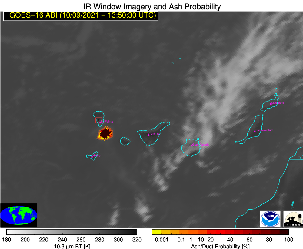
GOES-16 Ash Probability [click to play animation | MP4]
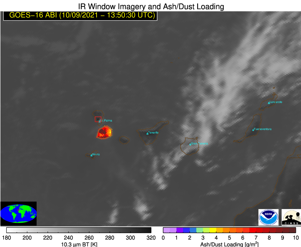
GOES-16 Ash Loading [click to play animation | MP4]
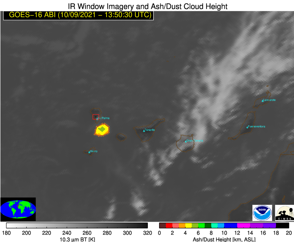
GOES-16 Ash Height [click to play animation | MP4]
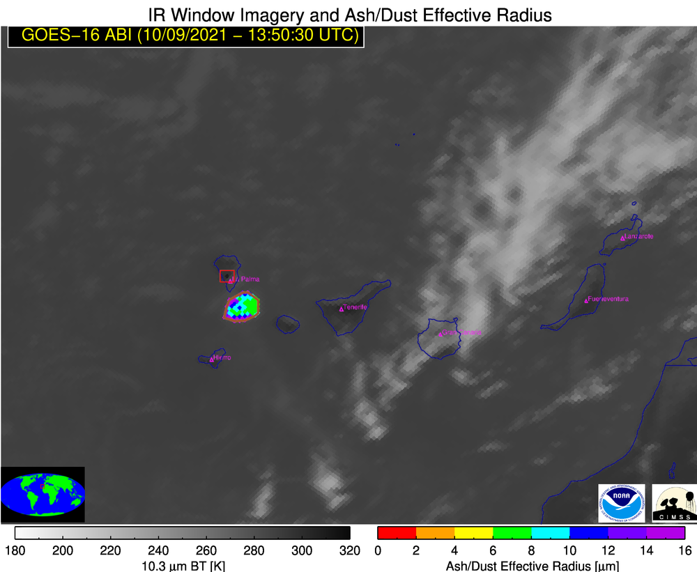
GOES-16 Ash Effective Radius [click to play animation | MP4]
View only this post
Read Less