Eastern Pacific Hurricane Rick, shown above near peak intensity at sunset on 17 October 2009, is the second strongest hurricanes on record in the eastern Pacific — weaker only than 1997’s Linda. Sustained winds at this time were estimated to be 180 miles per hour, and the central sea level... Read More
Eastern Pacific Hurricane Rick, shown above near peak intensity at sunset on 17 October 2009, is the second strongest hurricanes on record in the eastern Pacific — weaker only than 1997’s Linda. Sustained winds at this time were estimated to be 180 miles per hour, and the central sea level pressure was estimated to be 906 mb. Note in the visible imagery the presence of gravity waves in the cirrus shield that makes up the central dense overcast (CDO). In addition, as noted in the Tropical Prediction Center discussion issued near this time, the stadium effect in the Hurricane eye is readily apparent.
Rick formed out of a tropical disturbance southwest of the Gulf of Tehuantepec (a loop of 3-hourly water vapor imagery here, and a loop of 6-hourly 11-micron imagery here show an interesting flare-up of convection in the Gulf of Tehuantepec in the days before Rick formed. It is worth pondering how that convection influenced Rick’s early and rapid growth). The evolution from strong tropical depression (here, at 2100 UTC on 15 October) to minimal hurricane (here, at 1500 UTC on 16 October) to category 4 hurricane (here, at 1500 UTC on 17 October to category 5 hurricane, above, was rapid indeed and speaks to the ideal environment through which the disturbance traveled. Consider the image below from the CIMSS Tropical Weather Website.

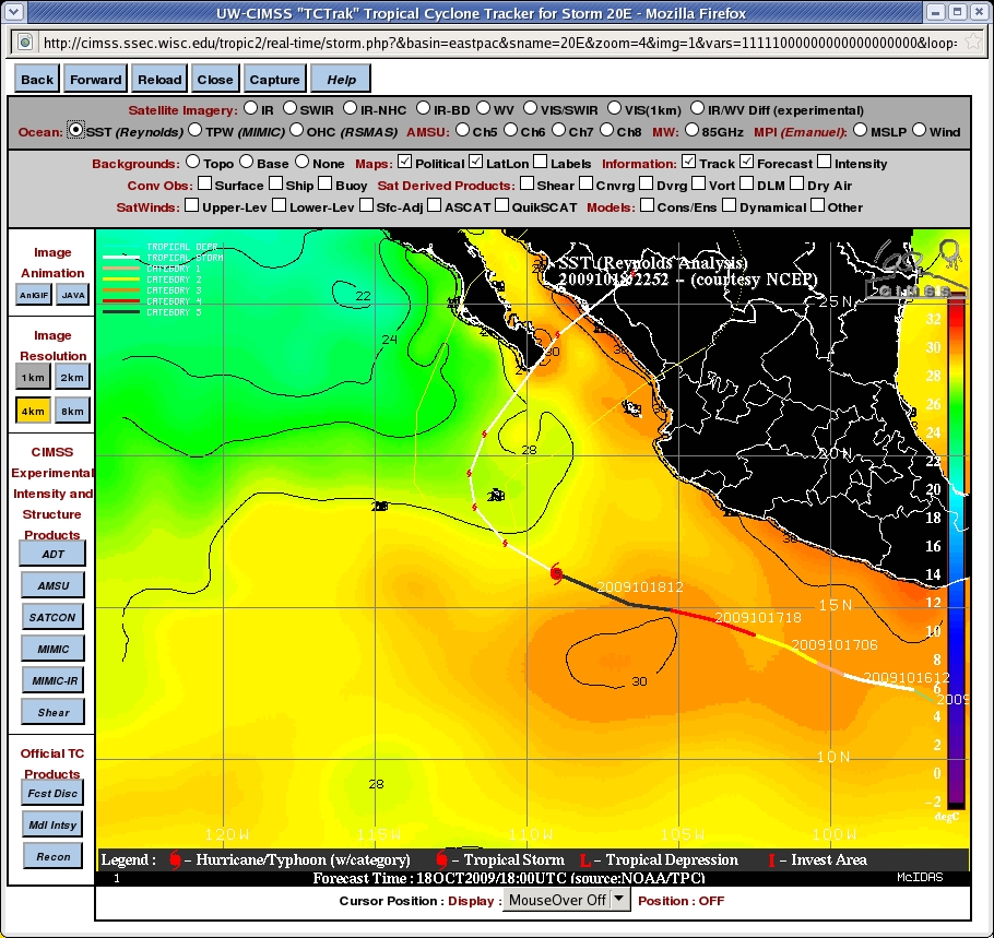
The image shows that the theoretical minimum to the central pressure in the region through which the system traveled was below 880 mb! (This value is a function of sea surface temperature, and of atmospheric thermodynamic profiles as described here. Note that Rick was moving across ocean waters with surface temperatures close to 30 C as it intensified rapidly. Wind shear as the storm rapidly intensified time was also very low (as diagnosed by Satellite winds). Very warm ocean waters and low vertical wind shear are key ingredients in allowing the strengthening of tropical systems.
The ideal environment resulted in a category 5 storm with a very tall circular ring of convection around the eye. The GOES-11 10.7-micron image, below, shows temperatures of nearly -80 C (the purple pixels within the grey) in the tallest convection around the eye.

(Added: Note in the water vapor and infrared imagery loops, above, the presence of what looks to be a binocular-shaped eye. This is an artifact of the interpolation used to blend GOES-12 and GOES-11 imagery to combine one cohesive picture. In individual images from either satellite, only a single eye is present).

Polar orbiting satellites, such as NOAA-19, give high-resolution images of the storm. The 10.8-micron example above, from 2020 UTC on 17 October, as the storm neared its peak intensity, shows pixels northwest of the storm center (this NOAA-19 pass is ascending, so north is towards the bottom of the image) with brightness temperatures of -84 C. Note also the more circular aspect ratio that comes from the polar-orbiter’s more top-down view, versus the Geostationary satellite’s oblique view. Visible imagery, below, at 0.65 and 0.86 microns, from the NOAA-19 AVHRR instrument, show better storm structure as well.


MODIS imagery from the Terra and Aqua satellites can also be used to investigate the storm. Unfortunately for this storm, the Aqua overpass granule split was right across the storm eye (granules are created so that the vast amount of data created by the satellite are more easily transportable). Gluing the two images together does not re-capture all the missed points, but it does give a good representation of the storm intensity here. A later MODIS image from TERRA, below, from 1755 UTC on 18 October (that is, about a day after the image from Aqua), below, shows a somewhat cloudier, but still quite distinct, eye. At this point, Rick has passed its peak in intensity.

(added: Jesse at Accu-Weather has other imagery of Rick here).
View only this post
Read Less
![GOES-7 Visible (0.65 um) images, 31 October and 01 November 1991 [click to play animation]](https://cimss.ssec.wisc.edu/satellite-blog/wp-content/uploads/sites/5/2009/10/911031-911101_goes7_visible_Halloween_storm_anim.gif)


")


