The first official GOES-15 full disk visible image (above) became available at 17:33 UTC on 06 April 2010. For more details, see the SSEC Spotlight and the NOAA News pages. GOES-15 (GOES-P) is the final spacecraft in the GOES N/O/P series — the next quantum leap in GOES satellite capabilities will come with the... Read More
")
GOES-15: first full disk visible image (click image to enlarge)
The first official GOES-15 full disk visible image (above) became available at 17:33 UTC on 06 April 2010. For more details, see the SSEC Spotlight and the NOAA News pages. GOES-15 (GOES-P) is the final spacecraft in the GOES N/O/P series — the next quantum leap in GOES satellite capabilities will come with the launch of GOES-R in 2015. GOES-R will include the improved 16-channel Advanced Baseline Imager (ABI).
The GOES-15 satellite will go through its post launch science test during the Summer of 2010.
A few close-up views from this GOES-15 full disk visible image (plus some comparisons between the 17:33 UTC image and the following 18:02 UTC image) are shown below:
")
Northern Hudson Bay and the Canadian Arctic Archipelago (showing some areas of ice-free water)

Frozen Lake Winnipeg in southern Manitoba, Canada

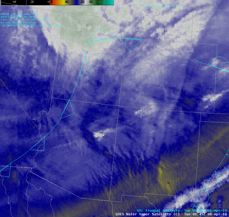
Cumulus development along a cold front in eastern Kansas
Within a few hours, the cumulus clouds seen forming along the cold front in eastern Kansas (above) developed into severe thunderstorms that produced hail up to 1.75 inch in diameter and wind gusts to 70 mph.

San Francisco Bay and the snow-covered Sierra Nevada mountains

Smoke plumes from small fires burning in the Florida panhandle region
The small fires producing smoke plumes seen in the Florida panhandle region (above) were but 3 of a large number of fires burning across the Southeast US on 06 April, according to the CIMSS Wildfire-ABBA product and the NOAA Hazards Mapping System product.

Smoke drifting northward across the southern Gulf of Mexico

Stratocumulus deck over the Rio Grande Valley region, with cirrus drifting overhead

Saharan dust blowing westward over the tropical Atlantic Ocean

Fingers of fog reaching into the valleys along the western slopes of the Andes in Chile

The center of a large cyclone in the South Pacific Ocean
Perhaps the most striking feature on the GOES-15 full disk visible image was the rather large cloud swirl associated with a cyclone located over the far southern portion of the South Pacific Ocean, west of the southern tip of South America (surface analysis). While it was large in size, it did not have access to a significant amount of moisture, as indicated by the MIMIC Total Precipitable Water product. A GOES-15 visible image close-up view of the center of the cyclone (above) showed the occluded front spiraling inward toward the center of the storm’s circulation.
")
GOES-11, GOES-15, GOES-13, and GOES-12 visible images (White Sands, NM)
Comparisons of visible images from GOES-11 (GOES-West), GOES-15, GOES-13, and GOES-12 (GOES-East) are shown for the White Sands, New Mexico area (above) and also for clouds with embedded convection producing precipitation over northern Iowa (below).
")
GOES-11, GOES-13, GOES-15, and GOES-12 visible images (northern Iowa)
View only this post
Read Less
")


")
")
")
