NOAK49 PAFG 110400 CCA
PNSAFG
AKZ222-111600-Public Information Statement…CORRECTED
National Weather Service Fairbanks AK
800 PM AKDT Sat Aug 10 2019…Lightning Detected within 300 Miles of North Pole Today…
A number of lightning strikes were recorded between 4pm and 6pm
today within 300 miles of the North Pole. The lightning strikes
occurred near 85 degrees north, 120 degrees east, which is about
700 miles north of the Lena River Delta of Siberia. This lightning
was detected by the GLD lightning detection network which is used
by the National Weather Service. This is one of the furthest
north lightning strikes in Alaska Forecaster memory.$$
JB
As noted by the NWS Fairbanks forecast office, lightning was detected with a thunderstorm located over the Arctic Ocean north of Siberia between 6-8 pm AKDT on 10 August (or 00-02 UTC on 11 August 2019). A sequence of AVHRR Visible (0.63 µm) and Infrared Window (10.8 µm) images from NOAA-15 (at 2315 UTC), NOAA-19 (at 0100 UTC) and NOAA-15 (at 0232 UTC) (below) showed the eastward motion of this thunderstorm, which had developed in advance of a 500 hPa lobe of vorticity — the coldest cloud-top infrared brightness temperature associated with this feature was -49.9ºC (yellow enhancement) at 0100 UTC.
![NOAA-19 AVHRR Visible (0.63 µm) and Infrared Window (10.8 µm) images [click to enlarge]](https://cimss.ssec.wisc.edu/satellite-blog/wp-content/uploads/sites/5/2019/08/190810_2315utc_noaa15_190811_0113utc_noaa19_0243utc_noaa15_visible_infrared_Arctic_lightning_anim.gif)
AVHRR Visible (0.63 µm) and Infrared Window (10.8 µm) images from NOAA-15 (at 2315 UTC), NOAA-19 (at 0100 UTC) and NOAA-15 (at 0232 UTC) [click to enlarge]
A number of lightning strikes were recorded Saturday evening (Aug. 10th) within 300 miles of the North Pole. The lightning strikes occurred near 85°N and 126°E. This lightning was detected by Vaisala’s GLD lightning detection network. #akwx pic.twitter.com/6jdxeMPBdH
— NWS Fairbanks (@NWSFairbanks) August 11, 2019
View only this post Read Less
![VIIRS True Color RGB and Infrared Window (11.45 µm) images from Suomi NPP and NOAA-20 [click to enlarge]](https://cimss.ssec.wisc.edu/satellite-blog/wp-content/uploads/sites/5/2019/08/190808_suomiNPP_noaa20_trueColor_infraredWindow_Typhoon_Lekima_anim.gif)
![Himawari-8 Infrared (10.4 µm) images [click to play animation| MP4]](https://cimss.ssec.wisc.edu/satellite-blog/wp-content/uploads/sites/5/2019/08/190807_190808_himawari8_infrared_Typhoon_Lekima_anim.gif)
![Himawari-8 "Clean" Infrared Window (10.4 µm) images, with contours and streamlines of deep-layer wind shear at 15 UTC [click to play animation]](https://cimss.ssec.wisc.edu/satellite-blog/wp-content/uploads/sites/5/2019/08/190808_himawari8_infrared_deepLayerWindShear_Lekima_anim.gif.gif)
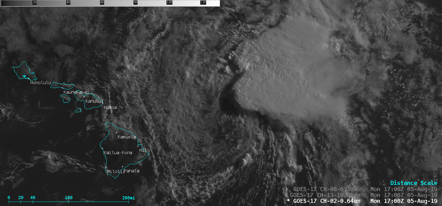
![GOES-15 Infrared Window (10.7 µm) images, with contours and streamlines of deep-layer wind shear [click to enlarge]](https://cimss.ssec.wisc.edu/satellite-blog/wp-content/uploads/sites/5/2019/08/190805_goes15_infrared_deepLayerShear_TD_Flossie_anim.gif)
![Visible images from GOES-17, GOES-15, GOES-14 and GOES-16, with SPC Storm Reports plotted in red [click to play animation | MP4]](https://cimss.ssec.wisc.edu/satellite-blog/wp-content/uploads/sites/5/2019/08/190803_goes17_goes15_goes14_goes16_visible_spcStormReports_ND_SD_anim.gif)
