CIMSS has hosted the MODIS Today website for many years. Its follow-on, the VIIRS Today has gone live as of 4 August 2020.As with MODIS today, the USA is subdivided into 8 sectors, and imagery on a 2-km, 1-km and 250-m grid is provided, even though VIIRS’ best resolution at nadir is 375... Read More

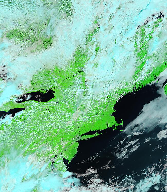
VIIRS Today imagery from 3 August (Daytime, left, True Color [Bands 1, 4, 3 from VIIRS] and False Color [Bands 7, 2, 1 from VIIRS] from Suomi NPP; Day Night Band imagery from NOAA-20, right)
has hosted the
MODIS Today website for many years. Its follow-on, the
VIIRS Today has gone live as of 4 August 2020.
As with MODIS today, the USA is subdivided into 8 sectors, and imagery on a 2-km, 1-km and 250-m grid is provided, even though VIIRS’ best resolution at nadir is 375 m (and 750 m for the Day Night Band).
The images above show True-Color and False Color imagery from Suomi NPP on shortly after noon on 3 August over the northeast United States, along with Day Night Band Imagery from NOAA-20, also from (the early morning of) 3 August, shortly before the Full Moon.
VIIRS Today does have an archive going back several years. The website allows you to choose either Suomi-NPP or NOAA-20 data (links at the page will also show you today’s Suomi-NPP and NOAA-20 orbital passes), and you can view True Color Imagery (combining channels only in the visible part of the electromagnetic spectrum), False-Color Imagery (combining visible and near-infrared information) or (unique to VIIRS) Day Night Band Imagery. There is also a link to a webpage showing the Moon Phase.
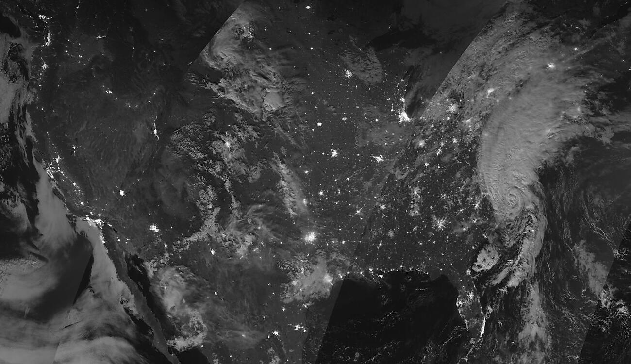
The image below, downloaded from VIIRS Today, shows the NOAA-20 Day Night Band composite from the morning of 4 August 2020 (link).
NOAA-20 Day Night Band image composite, 4 August 2020 (Click to enlarge)
View only this post
Read Less
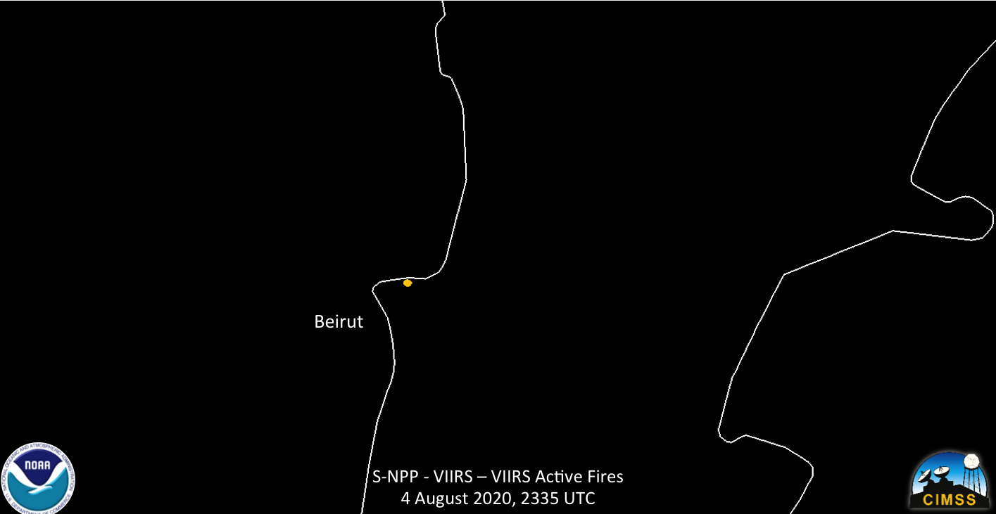
![Suomi NPP VIIRS Day/Night Band (0.7 µm), Near-Infrared (1.61 µm and 2.25 µm), Shortwave Infrared (3.75 µm) and Active Fires product (credit: William Straka. CIMSS) [click to enlarge]](https://cimss.ssec.wisc.edu/satellite-blog/images/2020/08/200804_2335utc_suomiNPP_viirs_dayNightBand_nearInfrared_shortwaveInfrared_viirsActiveFires_Beirut_Lebanon_fire_anim.gif)
![Plots of Spectral Response Functions for GOES-R series ABI 1..61 µm, 2.24 µm and 3.9 µm spectral bands [click to enlarge]](https://cimss.ssec.wisc.edu/satellite-blog/wp-content/uploads/sites/5/2018/08/ABI_Band_5_6_7_Spectral_Response_Functions_Fires.png)
![Meteosat-8 Visible (0.8 µm) images [click to enlarge]](https://cimss.ssec.wisc.edu/satellite-blog/images/2020/08/200804_meteosat8_visible_Beirut_explosion_anim.gif)
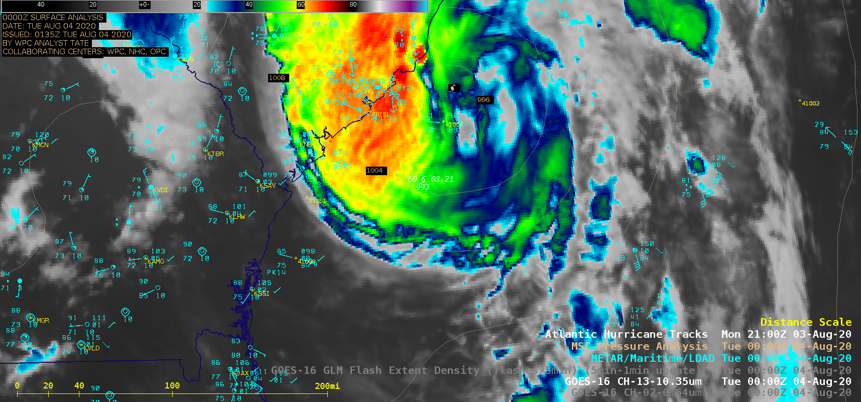
![GOES-16 “Red” Visible (0.64 µm) and “Clean” Infrared Window (10.35 µm) images [click to play animation | MP4]](https://cimss.ssec.wisc.edu/satellite-blog/images/2020/08/200803_goes16_visible_infrared_TS_Isaias_anim.gif)
![Plot of wind speed (blue), wind gust (red) and air pressure (green) at Buoy 41004 [click to enlarge]](https://cimss.ssec.wisc.edu/satellite-blog/images/2020/08/200804_02utc_buoy41004_wind_gust_pressure.png)
![GOES-16 “Clean” Infrared Window (10.35 µm) images, with and without an overlay of GLM Flash Extent Density [click to play animation | MP4]](https://cimss.ssec.wisc.edu/satellite-blog/images/2020/08/200803_goes16_infrared_glmFlashExtentDensity_TS_Isaias_anim.gif)
![VIIRS Day/Night Band (0.7 µm) images from Suomi NPP and NOAA-20 [click to enlarge]](https://cimss.ssec.wisc.edu/satellite-blog/images/2020/08/200804_suomiNPP_noaa20_viirs_dayNightBand_Isaias_anim.gif)
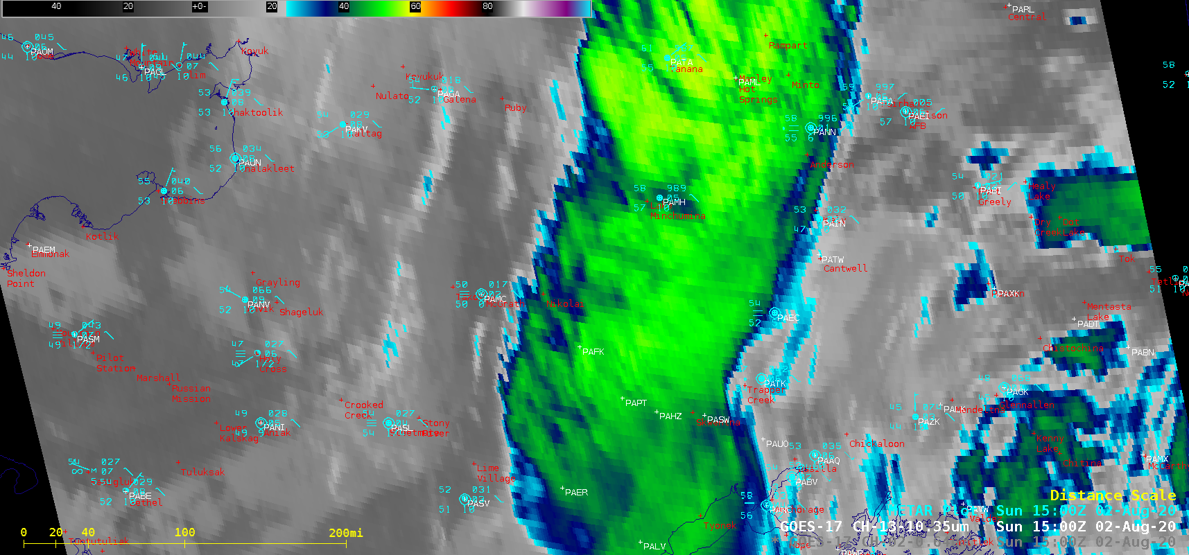
![Topography + GOES-17 "Clean" Infrared Window (10.35 µm) images [click to play animation | MP4]](https://cimss.ssec.wisc.edu/satellite-blog/images/2020/08/200802_goes17_infrared_AK_anim.gif)
![GOES-17 "Red" Visible (0.64 µm) images [click to play animation | MP4]]( https://cimss.ssec.wisc.edu/satellite-blog/images/2020/08/200802_goes17_visible_AK_anim.gif)
![Blended TPW and Percent of Normal TPW images [click to play animation | MP4]](https://cimss.ssec.wisc.edu/satellite-blog/images/2020/08/200801_200802_blendedTPW_percentNormalTPW_AK_anim.gif)
![VIIRS Infrared Window (11.45 ) images from NOAA-20 and Suomi NPP [click to enlarge]](https://cimss.ssec.wisc.edu/satellite-blog/images/2020/08/200802_noaa20_suomiNPP_viirs_infrared_AK_anim.gif)
