1-minute Mesoscale Domain Sector GOES-16 (GOES-East) “Red” Visible (0.64 µm) images (above) showed the eastward progression of a Mesoscale Convective System (MCS) that produced a long swath of damaging winds (SPC Storm Reports) or derecho from eastern Nebraska to Indiana on 10 August 2020. The highest measured wind gust was 112 mph in eastern Iowa at 1755 UTC.The corresponding... Read More
![GOES-16 “Red” Visible (0.64 µm) images, with SPC Storm Reports plotted in red [click to play animation | MP4]](https://cimss.ssec.wisc.edu/satellite-blog/images/2020/08/G16_M1_VIS_DERECHO_SPC_10AUG2020_B2_2020223_175527_GOES-16_0001PANEL_FRAME00227.GIF)
GOES-16 “Red” Visible (0.64 µm) images, with SPC Storm Reports plotted in red [click to play animation | MP4]
1-minute
Mesoscale Domain Sector GOES-16
(GOES-East) “Red” Visible (
0.64 µm) images
(above) showed the eastward progression of a Mesoscale Convective System (MCS) that produced a long swath of damaging winds (
SPC Storm Reports) or
derecho from eastern Nebraska to Indiana on
10 August 2020. The highest measured wind gust was 112 mph in eastern Iowa at 1755 UTC.
The corresponding GOES-16 “Clean” Infrared Window (10.35 µm) images are shown below.
![GOES-16 “Clean” Infrared Window (10.35 µm) images, with SPC Storm Reports plotted in cyan [click to play animation | MP4]](https://cimss.ssec.wisc.edu/satellite-blog/images/2020/08/G16_M1_IR_DERECHO_SPC_10AUG2020_B13_2020223_175527_GOES-16_0001PANEL_FRAME00227.GIF)
GOES-16 “Clean” Infrared Window (10.35 µm) images, with SPC Storm Reports plotted in cyan [click to play animation | MP4]
In a comparison of Infrared Window images from Suomi NPP (11.45 µm) and GOES-16 (10.35 µm) at 1931 UTC
(below), the higher spatial resolution of the VIIRS instrument detected infrared brightness temperatures as cold as -84ºC, compared to -76ºC with GOES-16 (the same color enhancement is applied to both images). The
northwest parallax offset associated with GOES-16 imagery at this location was also evident.
![Comparison of Infrared Window images from Suomi NPP (11.45 µm) and GOES-16 (10.35 µm) at 1931 UTC [click to enlarge]](https://cimss.ssec.wisc.edu/satellite-blog/images/2020/08/200810_1931utc_suomiNPP_goes16_infrared_WI_IL_anim.gif)
Comparison of Infrared Window images from Suomi NPP (11.45 µm) and GOES-16 (10.35 µm) at 1931 UTC [click to enlarge]
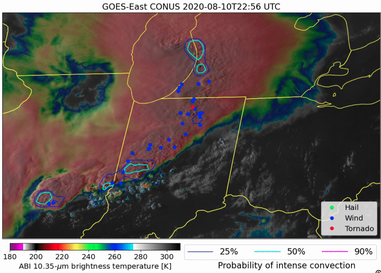
GOES-16 Visible/Infrared Sandwich Red-Green-Blue (RGB) and “Clean” Infrared Window (10.35 µm) images, with “probability of intense convection” contours and SPC Storm Reports, is shown below. The probability contours are produced from a deep-learning algorithm used to identify patterns in ABI and GLM imagery that correspond to intense convection. It is trained to highlight strong convection as humans would identify it. Work is ongoing to incorporate this storm-top information into
NOAA/CIMSS ProbSevere.
![GOES-16 Visible/Infrared Sandwich RGB and “Clean” Infrared Window (10.35 µm) images, with “probability of intense convection” contours and SPC Storm Reports (credit: John Cintineo, CIMSS) [click to play animation | MP4]](https://cimss.ssec.wisc.edu/satellite-blog/images/2020/08/derecho_capture.png)
GOES-16 Visible/Infrared Sandwich RGB and “Clean” Infrared Window (10.35 µm) images, with “probability of intense convection” contours and SPC Storm Reports (credit: John Cintineo, CIMSS) [click to play animation | MP4]
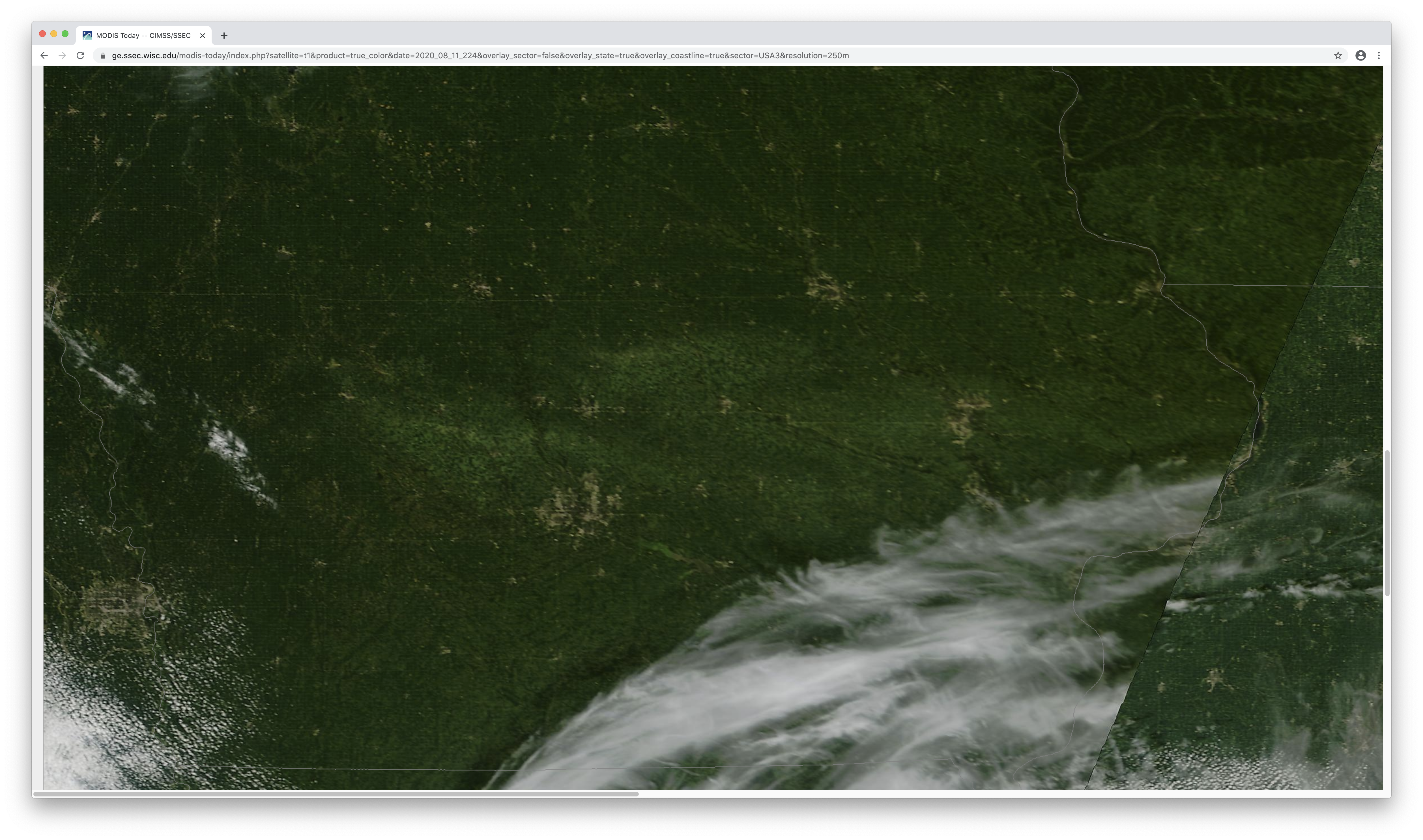
A comparison of Terra MODIS True Color RGB images (
source) from before (
28 July) and after (
11 August) the derecho
(below) revealed very large swaths of wind-damaged crops
(lighter shades of green) across Iowa. It is estimated that around 10 million acres of corn and soybean crops were flattened by the strong winds.
![Comparison of before (28 July) / after (11 August) Terra MODIS True Color RGB images centered over Iowa [click to enlarge]](https://cimss.ssec.wisc.edu/satellite-blog/images/2020/08/200728_200811_terra_modis_trueColorRGB_Iowa_derecho_crop_damage_anim.gif)
Comparison of before (28 July) / after (11 August) Terra MODIS True Color RGB images centered over Iowa [click to enlarge]
A toggle between VIIRS True Color RGB images from Suomi NPP and NOAA-20 visualized using
RealEarth (below) also displayed the crop damage swath.
![VIIRS True Color RGB images from Suomi NPP and NOAA-20 -- with and without map labels [click to enlarge]](https://cimss.ssec.wisc.edu/satellite-blog/images/2020/08/200811_suomiNPP_noaa20_viirs_trueColorRGB_IA_anim.gif)
VIIRS True Color RGB images from Suomi NPP and NOAA-20 — with and without map labels [click to enlarge]
Shown below is a before/after (28 July/11 August) comparison of VIIRS Day/Night Band (DNB) imagery (
source), where many of the areas across Iowa that suffered significant power outages — appearing darker (due to a lack of city lights) on the nighttime DNB images — corresponded to the large swaths of crop damage seen on the 11 August MODIS True Color image. Around 550,000 households lost power across the state.
![VIIRS Day/Night Band (0.7 µm) images on 28 July and 11 August, along with a MODIS True Color RGB image on 11 August [click to enlarge]](https://cimss.ssec.wisc.edu/satellite-blog/images/2020/08/200728_200811_viirs_dayNightBand_modis_trueColorRGB_IA_anim.gif)
VIIRS Day/Night Band (0.7 µm) images on 28 July and 11 August, along with a MODIS True Color RGB image on 11 August [click to enlarge]
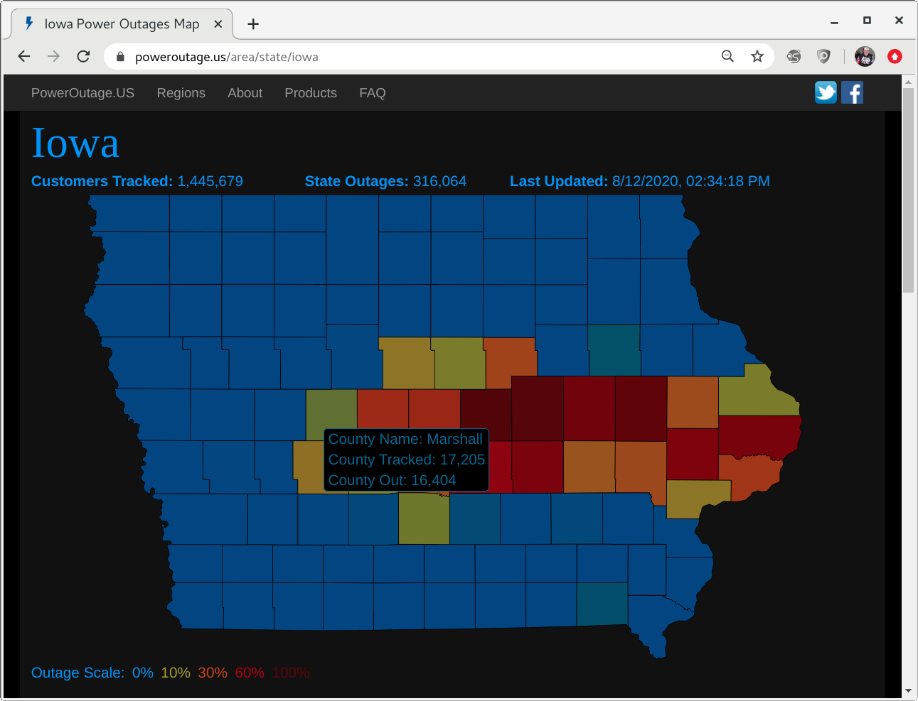
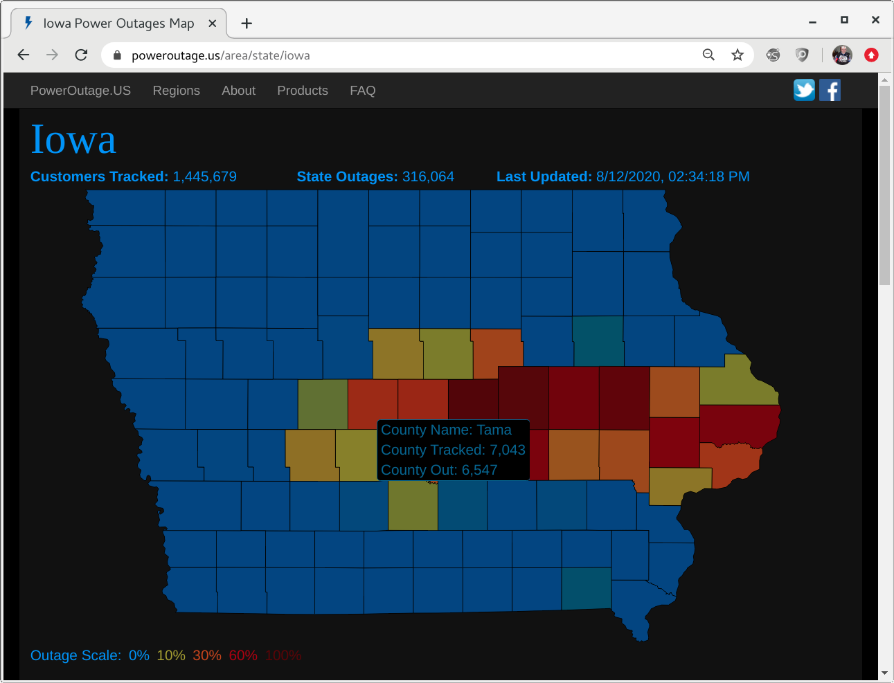
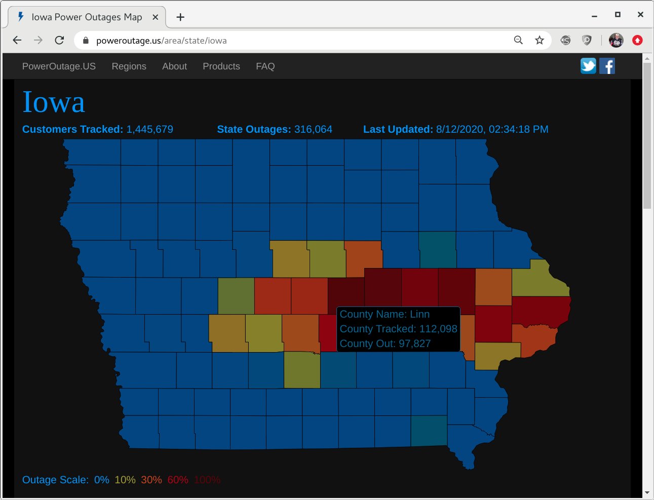
Even 2 days later (on 12 August), many customers remained without power across Iowa
(below), especially in
Marshall County (where peak winds of 106 mph were recorded),
Tama County (where peak winds of 90 mph were recorded) and
Linn County (where peak winds of 112 mph were recorded).
![Iowa counties with power outages on 12 August [click to enlarge]](https://cimss.ssec.wisc.edu/satellite-blog/images/2020/08/200812_IA_power_outages.png)
Iowa counties with power outages on 12 August [click to enlarge]
View only this post
Read Less
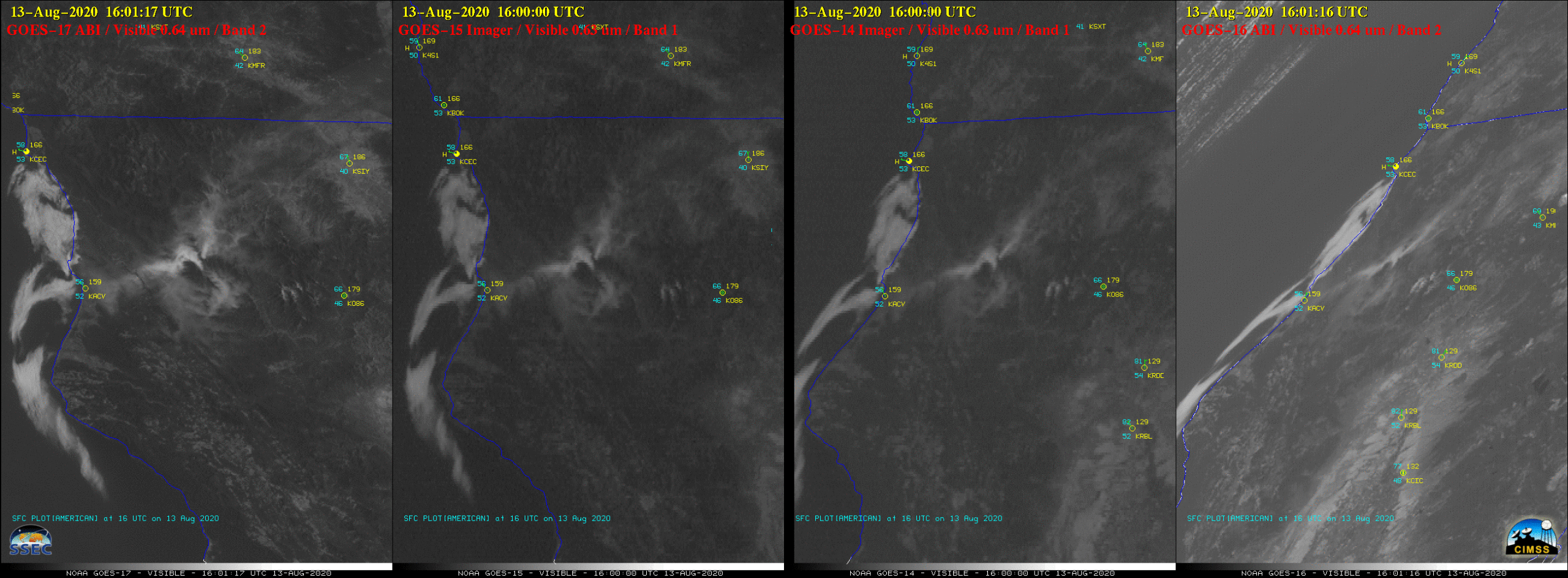
![From left to right, GOES-17, GOES-15, GOES-14 and GOES-16 Visible images [click to play animation | <a href="https://cimss.ssec.wisc.edu/satellite-blog/images/2020/08/200813_goes17_goes15_goes14_goes16_visible_RedSalmonComplex_wildfire_smoke_anim.mp4"><strong>MP4</strong></a>]](https://cimss.ssec.wisc.edu/satellite-blog/images/2020/08/200813_goes17_goes15_goes14_goes16_visible_RedSalmonComplex_wildfire_smoke_anim.gif)
![From left to right, GOES-17, GOES-15, GOES-14 and GOES-16 Shortwave Infrared images [click to play animation | MP4]](https://cimss.ssec.wisc.edu/satellite-blog/images/2020/08/200813_goes17_goes15_goes14_goes16_shortwaveInfrared_SoCal_fires_anim.gif)
![GOES-16 “Red” Visible (0.64 µm) images, with SPC Storm Reports plotted in red [click to play animation | MP4]](https://cimss.ssec.wisc.edu/satellite-blog/images/2020/08/200810_goes16_visible_spcStormReports_Midwest_Derecho_anim.gif)
![GOES-16 “Clean” Infrared Window (10.35 µm) images, with SPC Storm Reports plotted in cyan [click to play animation | MP4]](https://cimss.ssec.wisc.edu/satellite-blog/images/2020/08/200810_goes16_infrared_spcStormReports_Midwest_Derecho_anim.gif)
![GOES-16 Visible/Infrared Sandwich RGB and “Clean” Infrared Window (10.35 µm) images, with “probability of intense convection” contours and SPC Storm Reports (credit: John Cintineo, CIMSS) [click to play animation | MP4]](https://cimss.ssec.wisc.edu/satellite-blog/images/2020/08/derecho_20200810.GIF)

![Himawari-8 True Color RGB images [click to play animation | MP4]](https://cimss.ssec.wisc.edu/satellite-blog/images/2020/08/200810_himawari8_trueColorRGB_Sinabung_anim.gif)
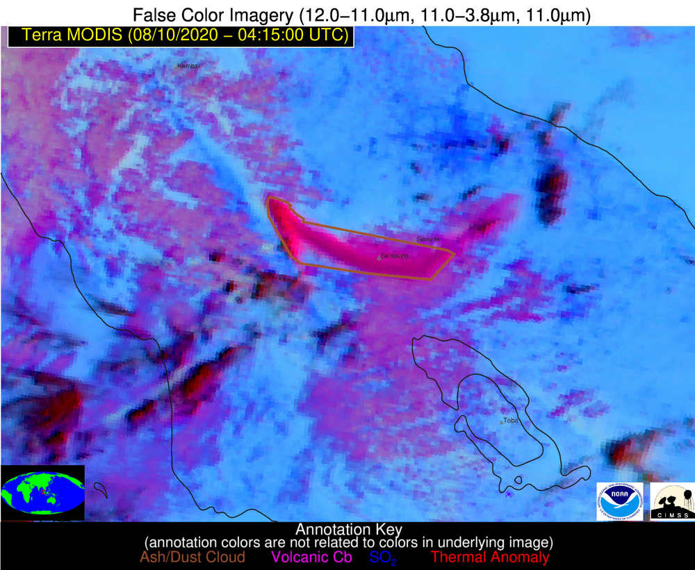
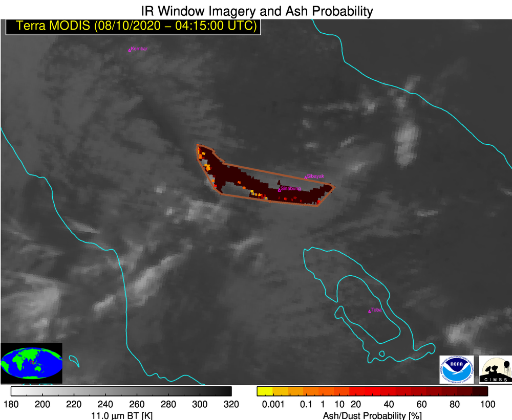
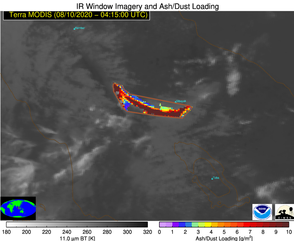
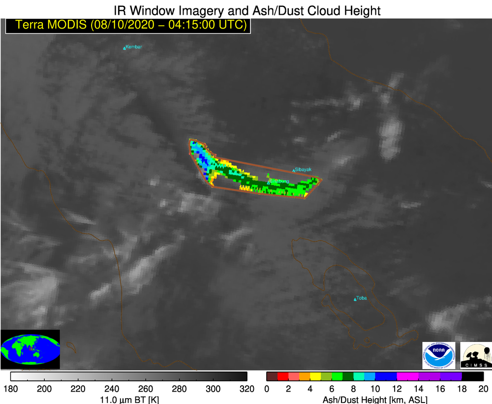
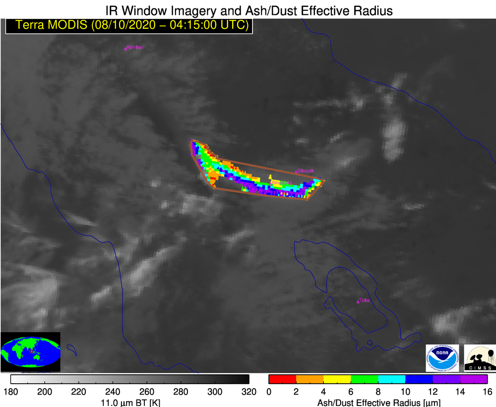
![Terra MODIS False Color RGB, Ash Probability, Ash Loading, Ash Height and Ash Effective Radius [click to enlarge]](https://cimss.ssec.wisc.edu/satellite-blog/images/2020/08/200810_0415utc_terra_modis_falseColorRGB_ashProbabilty_ashLoading_ashHeight_ashEffectiveRadius_Sinabung_anim.gif)
![Plot of 00 UTC rawinsonde data from Medan, Indonesia [click to enlarge]](https://cimss.ssec.wisc.edu/satellite-blog/images/2020/08/200810_00UTC_WIMM_RAOB.GIF)
![GOES-16 True Color RGB images [click to play animation | MP4]](https://cimss.ssec.wisc.edu/satellite-blog/images/2020/08/200809_goes16_trueColorRGB_Brazil_smoke_anim.gif)
