GOES-16 (GOES-East) “Red” Visible (0.64 µm), Shortwave Infrared (3.9 µm) and “Clean” Infrared Window (10.35 µm) images (above) showed 2 pulses of pyro-convection emanating from the Williams Fork Fire that was burning between between Kremmling (K20V) and Berthoud Pass (K0CO) in Colorado on 14 August 2020. The cloud of the second pulse, originating around 2300 UTC, exhibited... Read More
![GOES-16 “Red” Visible (0.64 µm, top), Shortwave Infrared (3.9 µm, center) and “Clean” Infrared Window (10.35 µm, bottom) images, with hourly plots of surface reports [click to play animation | MP4]](https://cimss.ssec.wisc.edu/satellite-blog/images/2020/08/G16_VIS_SWIR_IR_CO_PYROCB_14AUG2020_B2713_2020228_002616_0003PANELS_FRAME00042.GIF)
GOES-16 “Red” Visible (0.64 µm, top), Shortwave Infrared (3.9 µm, center) and “Clean” Infrared Window (10.35 µm, bottom) images, with hourly plots of surface reports [click to play animation | MP4]
GOES-16
(GOES-East) “Red” Visible (
0.64 µm), Shortwave Infrared (
3.9 µm) and “Clean” Infrared Window (
10.35 µm) images
(above) showed 2 pulses of pyro-convection emanating from the
Williams Fork Fire that was burning between between Kremmling (K20V) and Berthoud Pass (K0CO) in Colorado on
14 August 2020. The cloud of the second pulse, originating around 2300 UTC, exhibited infrared brightness temperatures of -40ºC and colder
(shades of blue in the 10.35 µm images) — assuring the heterogeneous nucleation of all supercooled water droplets to form ice crystals, and thereby meeting the criteria of a pyrocumulonimbus (pyroCb). The pyroCb then drifted east-southeastward across Colorado.
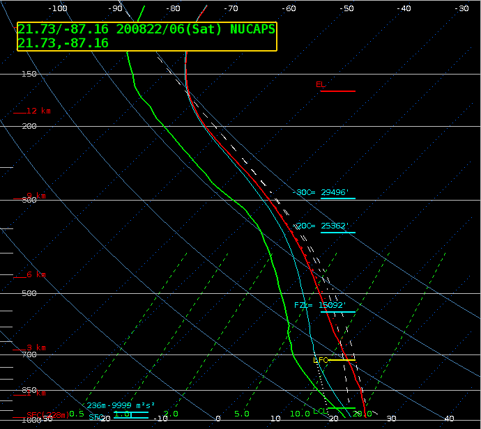
The coldest pyroCb infrared brightness temperature was -46ºC, which corresponded to an altitude near 11 km according to rawinsonde data from Denver (below).
![Plot of rawinsonde data from Denver [click to enlarge]](https://cimss.ssec.wisc.edu/satellite-blog/images/2020/08/200815_00UTC_KBOU_RAOB.GIF)
Plot of rawinsonde data from Denver [click to enlarge]
===== 15 August Update =====
![GOES-16 “Red” Visible (0.64 µm, top), Shortwave Infrared (3.9 µm, center) and “Clean” Infrared Window (10.35 µm, bottom) images, with hourly plots of surface reports [click to play animation | MP4]](https://cimss.ssec.wisc.edu/satellite-blog/images/2020/08/G16_VIS_SWIR_IR_CO_PYROCB_15AUG2020_B2713_2020228_233054_0003PANELS_FRAME00211.GIF)
GOES-16 “Red” Visible (0.64 µm, top), Shortwave Infrared (3.9 µm, center) and “Clean” Infrared Window (10.35 µm, bottom) images, with hourly plots of surface reports [click to play animation | MP4]
On the following day, 1-minute
Mesoscale Domain Sector GOES-16
(GOES-East) Visible, Shortwave Infrared and Infrared images
(above) showed another pyroCb that developed around 2240 UTC. This pyroCb moved southeastward, exhibiting cloud-top infrared brightness temperatures as cold as -55ºC — which, according to
rawinsonde data from Denver
(below) represented an altitude near 12 km.
![Plot of 00 UTC rawinsonde data from Denver [click to enlarge]](https://cimss.ssec.wisc.edu/satellite-blog/images/2020/08/200816_00UTC_KDNR_RAOB.GIF)
Plot of 00 UTC rawinsonde data from Denver [click to enlarge]
Farther to the west, the
Loyalton Fire was burning in northern California, near the border with Nevada. 1-minute Mesoscale Domain Sector GOES-17
(GOES-West) Visible, Shortwave Infrared, Infrared Window and
Fire Temperature Red-Green-Blue (RGB) images
(below) showed that this fire produced a pyroCb cloud around 2100 UTC, which then drifted northeastward across the California/Nevada border.
![GOES-17 Visible (0.64 µm, top left), Shortwave Infrared (3.9 µm, top right), Infrared Window (10.35 µm, bottom left) and Fire Temperature RGB (bottom right) [click to play animation | MP4]](https://cimss.ssec.wisc.edu/satellite-blog/images/2020/08/ca_4panel-20200815_213555.png)
GOES-17 Visible (0.64 µm, top left), Shortwave Infrared (3.9 µm, top right), Infrared Window (10.35 µm, bottom left) and Fire Temperature RGB (bottom right) [click to play animation | MP4]
This event exhibited extreme fire behavior, producing fire whirls and prompting NWS Reno to issue a
Tornado Warning for the source region of the pyroCb at 2135 UTC. The cloud-top infrared brightness temperatures of the pyroCb were around -55ºC; rawinsonde data from Reno
(below) indicated that this corresponded to an altitude near 12 km.
![Plot of 00 UTC rawinsonde data from Reno [click to enlarge]](https://cimss.ssec.wisc.edu/satellite-blog/images/2020/08/200816_00UTC_KREV_RAOB.GIF)
Plot of 00 UTC rawinsonde data from Reno [click to enlarge]
View only this post
Read Less

![Suomi NPP VIIRS Day/Night Band (0.7 µm) and Near-Infrared (1.61 µm and 2.25 µm) images along with the VIIRS Active Fires product (credit: William Straka, CIMSS) [click to enlarge]](https://cimss.ssec.wisc.edu/satellite-blog/images/2020/08/200820_1002utc_suomiNPP_viirs_dayNightBand_shortwaveInfrared_nearInfrared_viirsAcitiveFires_Northern_CA_anim.gif)
![GOES-17 Fire Temperature RGB and "Red" Visible (0.64 µm) images [click to play animation | MP4]](https://cimss.ssec.wisc.edu/satellite-blog/images/2020/08/200820_goes17_fireTemperatureRGB_visible_CA_wildfires_anim.gif)
![GOES-17 True Color RGB images [click to play animations | MP4]](https://cimss.ssec.wisc.edu/satellite-blog/images/2020/08/200820_goes17_trueColorRGB_CA_wildfire_smoke_zoom_anim.gif)
![GOES-16 “Red” Visible (0.64 µm) and “Clean” Infrared Window (10.35 µm) images [click to play animation | MP4]](https://cimss.ssec.wisc.edu/satellite-blog/images/2020/08/200818_goes16_visible_infrared_Hurricane_Genevieve_anim.gif)
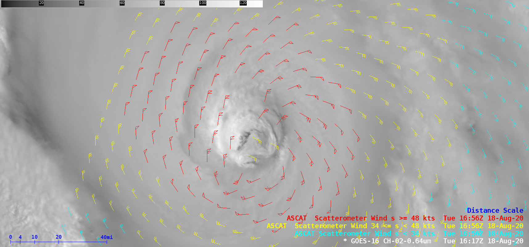
![GOES-16 “Red” Visible (0.64 µm) image, with plots of ASCAT scatterometer surface winds [click to enlarge]](https://cimss.ssec.wisc.edu/satellite-blog/images/2020/08/genevieve_vis_ascat-20200818_161755.png)
![GOES-16 “Red” Visible (0.64 µm, top), Shortwave Infrared (3.9 µm, center) and “Clean” Infrared Window (10.35 µm, bottom) images, with hourly plots of surface reports [click to play animation | MP4]](https://cimss.ssec.wisc.edu/satellite-blog/images/2020/08/200814_goes16_visible_shortwaveInfrared_longwaveInfraredWindow_CO_pyroCb_anim.gif)
![GOES-16 “Red” Visible (0.64 µm, top), Shortwave Infrared (3.9 µm, center) and “Clean” Infrared Window (10.35 µm, bottom) images, with hourly plots of surface reports [click to play animation | MP4]](https://cimss.ssec.wisc.edu/satellite-blog/images/2020/08/200815_goes16_visible_shortwaveInfrared_longwaveInfraredWindow_CO_pyroCb_anim.gif)
![GOES-17 Visible (0.64 µm, top left), Shortwave Infrared (3.9 µm, top right), Infrared Window (10.35 µm, bottom left) and Fire Temperature RGB (bottom right) [click to play animation | MP4]](https://cimss.ssec.wisc.edu/satellite-blog/images/2020/08/200815_goes17_visible_shortwaveInfrared_infraredWindow_fireTemperatureRGB_Loyalton_Fire_anim.gif)
