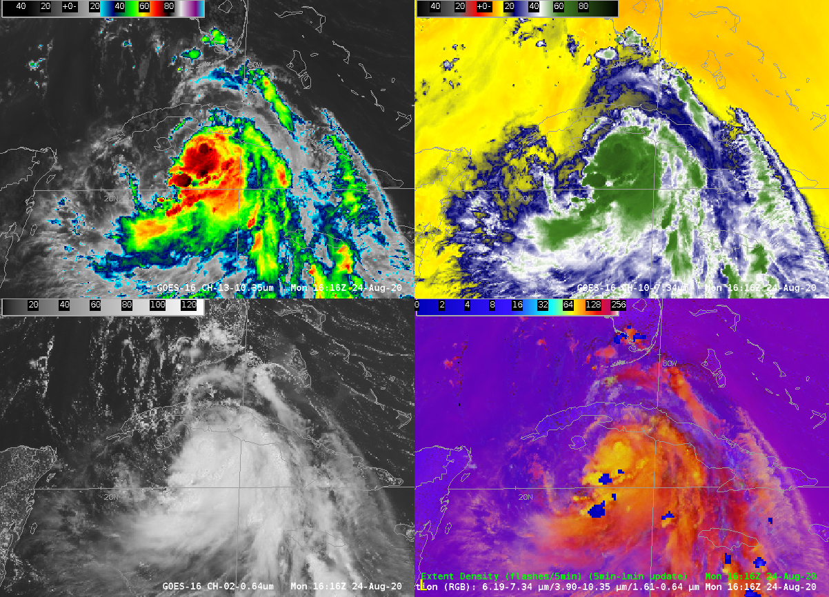

GOES-16 4-panel display over Tropical Storm Laura, 0946 to 1621 UTC On 24 August 2020 (Click to animate); Upper Left: Band 13 “Clean Window” infrared (10.3 µm); Upper Right, Band 10 Low-level Water vapor infrared (7.3 µm); Lower Left: Band 2 Red Visible (0.64 µm); Lower Right, Day Convection RGB overlain with 5-minute aggregate GLM Flash Extent Density
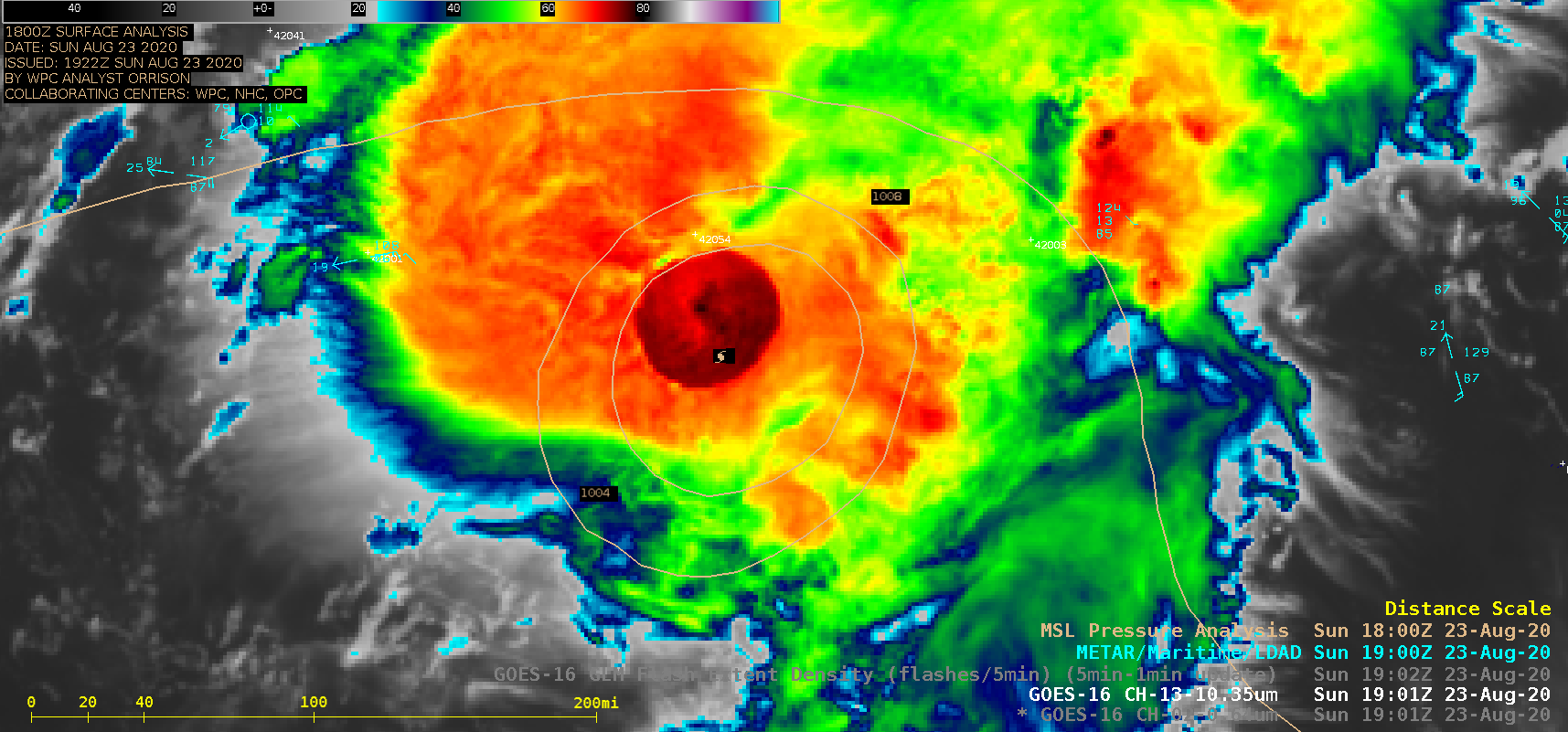
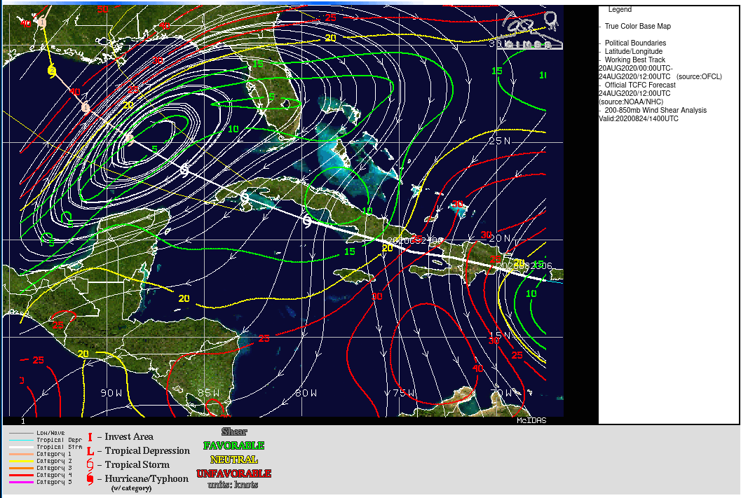
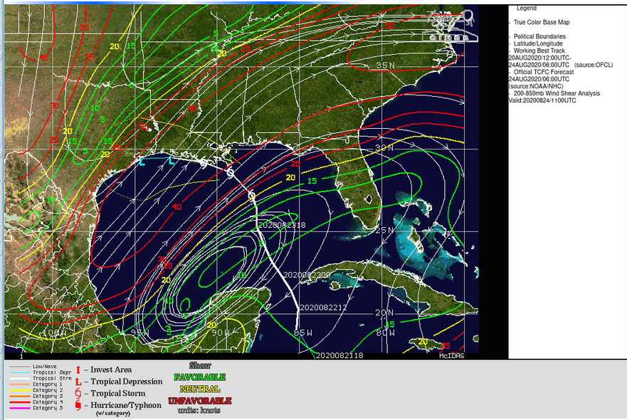
Tropical Storm Laura’s path near/over the Greater Antilles has affected her strength, and the relative lack of organization means that night-time satellite identification of the center is a challenge. Consider the animation above. Northerly shear (analysis from this site) has shifted the coldest cloud tops to the south of the circulation center and with the 5-minute routine CONUS imagery, it is difficult to discern a surface circulation along the south coast of Cuba, where it was moving. (A cluster of convection does appear there, although it is initially dwarfed in size by the convection to the south, south of 20 Latitude)
Visible imagery that becomes available at sunrise does show the center. The center gains prominence in the infrared as well as the convection to the south weakens. Note that the center can be discerned within the 1-minute shortwave infrared (3.9 µm) imagery from GOES-16 Mesoscale Sector 1: this link shows data from 0702 to 0803 UTC. In the greyscale enhancement used in the linked-to animation, coldest cloud tops appear black and speckled because of a lack of precision at very cold temperatures in the 3.9 µm channel).
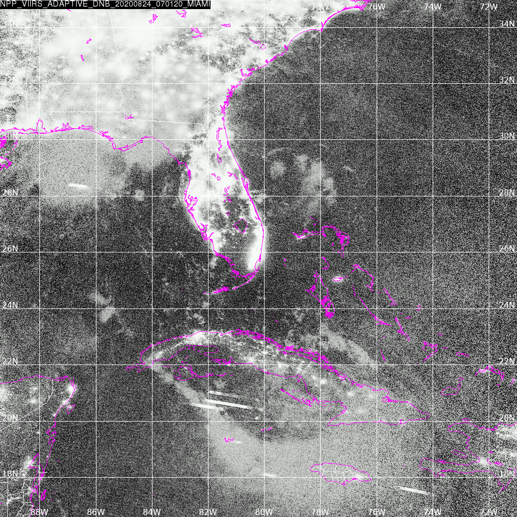
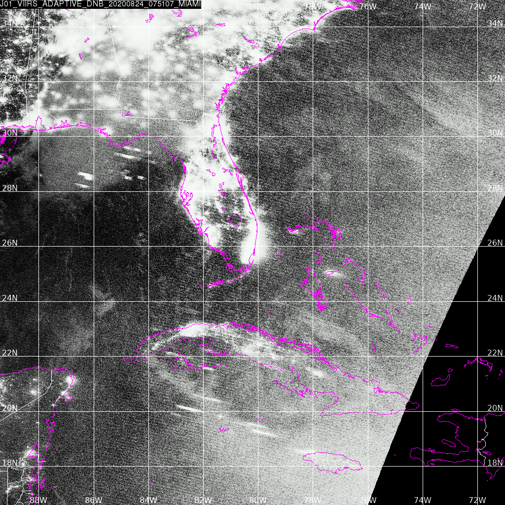
Sometimes, Day Night Band imagery from VIIRS can be useful in identifying tropical cyclone centers at night (see these 2016 examples with Matthew and Karl, for example). On the morning of 24 August, however, reflected moonlight was nil (Moonset over Cuba today was around 0500 UTC); in addition, the NOAA-20 overpass had Laura near the edge of the scan. Adaptive DNB imagery from Suomi NPP (just after 0700 UTC) and NOAA-20 (just before 0800 UTC), from the Direct Broadcast site at AOML in Miami, do show low clouds just south of Cuba, near the Jardines de la Reina, but it is a challenge to identify a surface circulation from this DNB imagery.
Suomi-NPP and NOAA-20 VIIRS Day Night Band Imagery at 0701 and 0752 UTC on 24 August 2020 (Click to enlarge)
Interests in Cuba and along the Gulf Coast of the United States should monitor closely the progress of Laura. Refer to the National Hurricane Center website for the latest forecasts.
View only this post Read Less


![GOES-17 “Red” Visible (0.64 µm), Shortwave Infrared (3.9 µm) and “Clean” Infrared Window (10.3 µm) images [click to play animation | MP4]](https://cimss.ssec.wisc.edu/satellite-blog/images/2020/08/200823_goes17_visible_shortwaveInfrared_infrared_Castle_Fire_CA_pyrocb_anim.gif)
![Plot of 00 UTC rawinsonde data from Las Vegas, NV [click to enlarge]](https://cimss.ssec.wisc.edu/satellite-blog/images/2020/08/200824_00UTC_KVEF_RAOB.GIF)
![GOES-16 “Red” Visible (0.64 µm) and “Clean” Infrared Window (10.35 µm) images (with and without an overlay of GLM Flash Extent Density) [click to play animation | MP4]](https://cimss.ssec.wisc.edu/satellite-blog/images/2020/08/200823_goes16_visible_infrared_glmFlashExtentDensity_Hurricane_Marco_anim.gif)
![Infrared images from Suomi NPP and GOES-16 [click to enlarge]](https://cimss.ssec.wisc.edu/satellite-blog/images/2020/08/200823_1842utc_suomiNPP_goes16_infrared_Hurricane_Marco_anim.gif)
