Researchers from NOAA and UW-CIMSS have developed an experimental model that predicts the “probability of intense convection” inferred from GOES ABI and GLM fields. The model is a convolutional neural network, which carries the assumption that the inputs are images and have spatial context. It is a great tool for image... Read More
Researchers from NOAA and UW-CIMSS have developed an experimental model that predicts the “probability of intense convection” inferred from GOES ABI and GLM fields. The model is a convolutional neural network, which carries the assumption that the inputs are images and have spatial context. It is a great tool for image classification.
GOES-16 ABI CH02 reflectance (a visible channel), ABI CH13 brightness temperature (an infrared window channel [IR]), and GLM flash extent density (FED; generated using glmtools), were used as inputs to the model. The model learned important features that have been traditionally difficult or expensive to code into an algorithm, such as pronounced overshooting tops (OTs), enhanced-V features, thermal couplets, above-anvil cirrus plumes (AACPs), strong brightness temperature gradients, cloud-top divergence, and texture from visible reflectance.
It is hoped that such a model may be able to one day:
- provide earlier notice of developing or decaying intense convection
- provide guidance in regions with no weather radars
- provide a quantitative way to leverage 1-min mesoscale scans
- ultimately improve the accuracy and lead time of severe weather warnings
The model is very experimental and is not yet running in real-time. The remainder of this post catalogues some examples of the deployed model on select scenes.
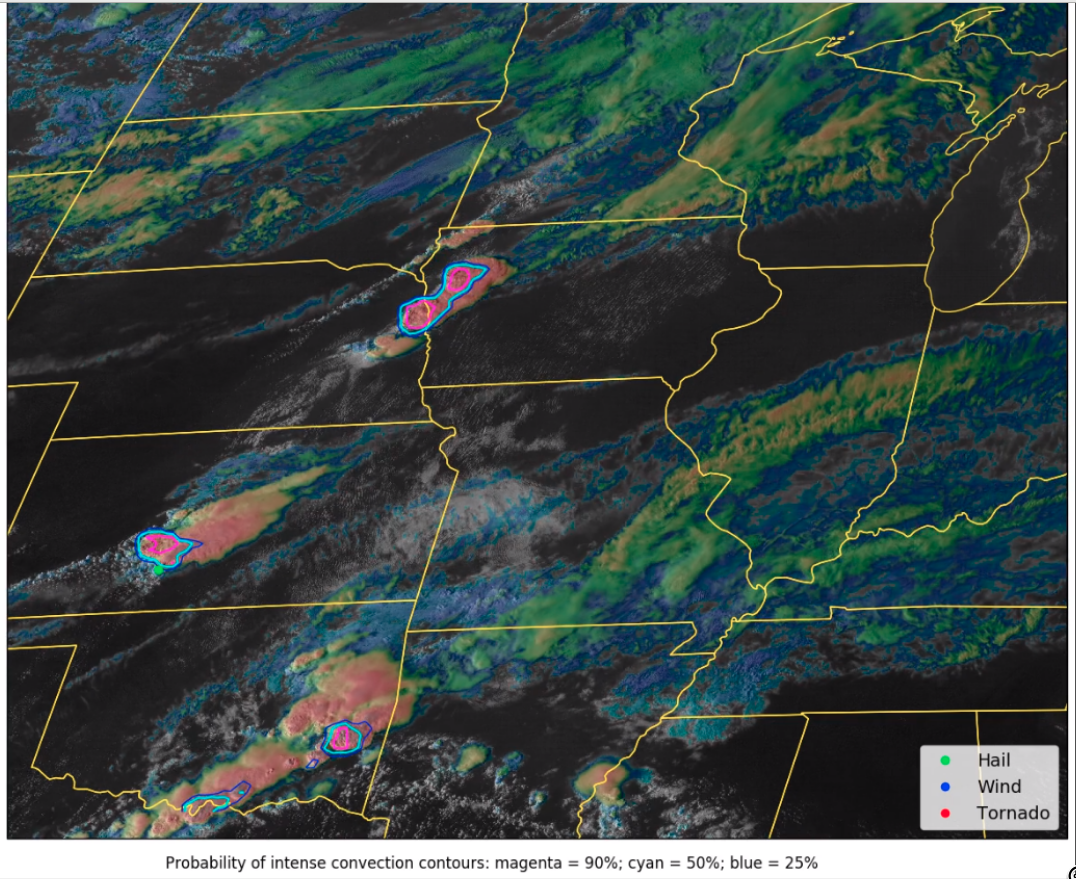
The movies below use as a background the CH02-CH13 “sandwich” product, whereby cloud-top 11-µm brightness temperature and 0.64-µm reflectance can be seen in tandem. This generally helps observers see how changes in storm-top structure correlate with changes in 11-µm brightness temperature. A grid of “probability of intense convection” was generated for each scene with a moving 32×32 pixel window (each pixel = ~2 km), with the model generating one probability for each window. These probabilities were then contoured with the 25%, 50%, and 90% contours as blue, cyan, and magenta. Preliminary severe local storm reports from the SPC rough log are also plotted as circles.
The example below shows that the model handled two separate severe wind threats in Missouri, identifying cold cloud top regions in the IR that also looked “bubbly” from the visible channel. As the sun was setting, a cold front lit up with very intense convection from Oklahoma through Missouri. Again, the model did a decent job highlighting the strongest areas of convection which correlated well with severe local storm reports. It should also be noted that the model does not seem to have significantly degraded output when the visible channel is missing (after sunset).
The next example is at a higher satellite viewing angle in western Nebraska, western South Dakota, and eastern Wyoming. The model again does a good job highlighting the strongest areas of storms. It should be noted that not every identified region has severe reports and not every severe report has a probability of intense convection ? 25%, but that there is generally good correspondence between reports and the model probabilities nonetheless.
This example is from the Southeast U.S. in more of a low-shear “microburst” environment instead of a high-shear “supercell” environment. You can see that instead of predicting high probabilities for all of the convective storms, the model exhibits the highest probabilities for the storm clusters that at least subjectively look the strongest.
This next example from the Central Plains demonstrates the ability to discern decaying convection, as the first storm moves into Missouri and then quickly diminishes in appearance and in probability. It also demonstrates the model’s ability to pick out multiple threat areas within a large cloud mass at night.
This is an example using mesoscale scans. Despite not being trained with 1-min data, the model predictions still look very fluid and reasonable. This could be an excellent way for scientists and forecasters to leverage 1-min observations in a quantitative manner.
Another example using GOES-East 1-min mesoscale scans. The model generally picks out the strongest portions of a MCS in Illinois and Indiana.
At a very high viewing angle, the model predicts probabilities of ?90% for a storm in Arizona. The storm did not generate severe reports, but was warned on by the NWS multiple times.
The model is deployed during an early autumn severe weather outbreak.
This example shows the model deployed on 1-min mesoscale scans over very intense thunderstorms in Argentina. It demonstrates that the model is generally applicable to anywhere in the world where advanced imager and GLM-like observations are present.
Here, a model was trained without GLM data and deployed for an example in the Alaska Panhandle, where GLM data is not available. This storm prompted a severe thunderstorm warning from the Juneau, AK NWS office. Note the change in the values of the probability contours. The maximum probability for this storm was 36% at 02:43 UTC. In a relative sense, the intense convection probability product could still be useful in unconventional regions, such as Alaska.
View only this post
Read Less
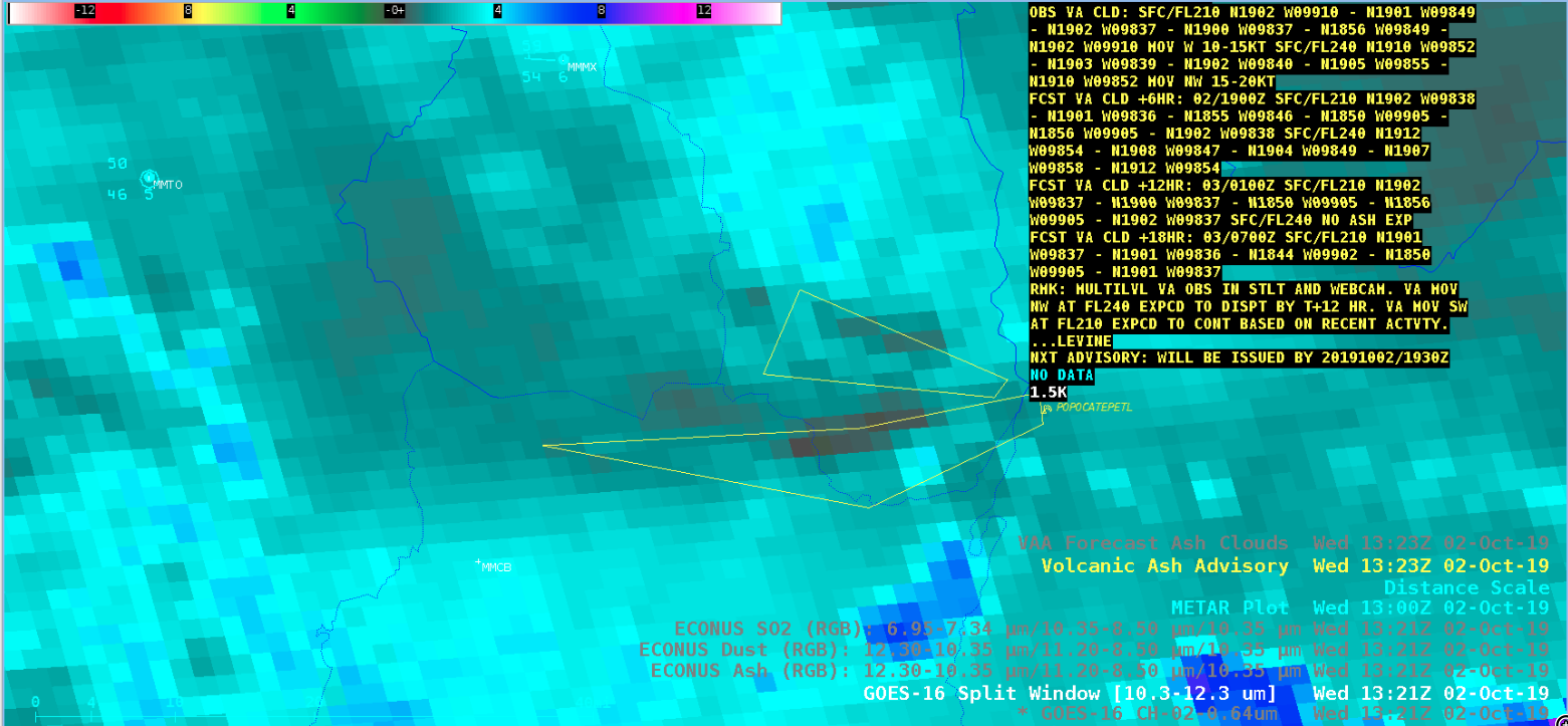

![GOES-16 Split Window image with the text of the 1323 UTC Volcanic Ash Advisory [click to enlarge]](https://cimss.ssec.wisc.edu/satellite-blog/wp-content/uploads/sites/5/2019/10/191002_1321utc_goes16_swd_vaa_popo.png)
![GOES-16 Volcanic Ash Height product [click to play animation | MP4]](https://cimss.ssec.wisc.edu/satellite-blog/wp-content/uploads/sites/5/2019/10/191002_goes16_ash_height_Popo_anim.gif)

![GOES-16 Day Cloud Phase Distinction RGB images [click to play animation | MP4]](https://cimss.ssec.wisc.edu/satellite-blog/wp-content/uploads/sites/5/2019/09/190930_goes16_dayCloudPhaseDistinctionRGB_MT_anim.gif)
![GOES-16 Mid-level Water Vapor images, with hourly plots of precipitation type [click to play animation | MP4]](https://cimss.ssec.wisc.edu/satellite-blog/wp-content/uploads/sites/5/2019/09/190928_190930_goes16_waterVapor_precipitationType_Northern_Rockies_snowstorm_anim.gif)
![GOES-16 Day Cloud Phase Distinction and Day Snow-Fog RGB images [click to play animation | MP4]](https://cimss.ssec.wisc.edu/satellite-blog/wp-content/uploads/sites/5/2019/10/191001_goes16_dayCloudPhaseDistinctionRGB_daySnowFogRGB_MT_anim.gif)
![GOES-16 Day Cloud Phase Distinction RGB and Topography images [click to enlarge]](https://cimss.ssec.wisc.edu/satellite-blog/wp-content/uploads/sites/5/2019/10/191001_goes16_dayCloudPhaseDistinctionRGB_topography_MT_AB_anim.gif)
![GOES-16 "Clean" Infrared Window (10.35 µm) images [click to play animation | MP4]](https://cimss.ssec.wisc.edu/satellite-blog/wp-content/uploads/sites/5/2019/09/190928_goes16_infrared_Lorenzo_anim.gif)
![Plot of the CIMSS Advanced Dvorak Technique (ADT) for Hurricane Lorenzo [click to enlarge]](https://cimss.ssec.wisc.edu/satellite-blog/wp-content/uploads/sites/5/2019/09/190929_adt_Lorenzo.GIF)
![GOES-16 Water Vapor images, with contours and streamlines of deep-layer wind shear [click to play animation]](https://cimss.ssec.wisc.edu/satellite-blog/wp-content/uploads/sites/5/2019/09/190927_190929_goes16_waterVapor_deepLayerShear_anim.gif)
![Sea Surface Temperature and Ocean Heat Content on 29 September, with a plot of the track/intensity of Lorenzo [click to enlarge]](https://cimss.ssec.wisc.edu/satellite-blog/wp-content/uploads/sites/5/2019/09/190929_seaSurfaceTemperature_oceanHeatContent_Lorenzo_anim.gif)
