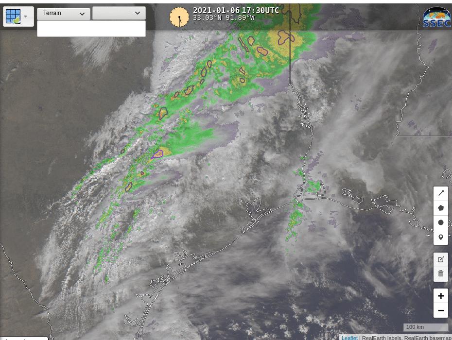
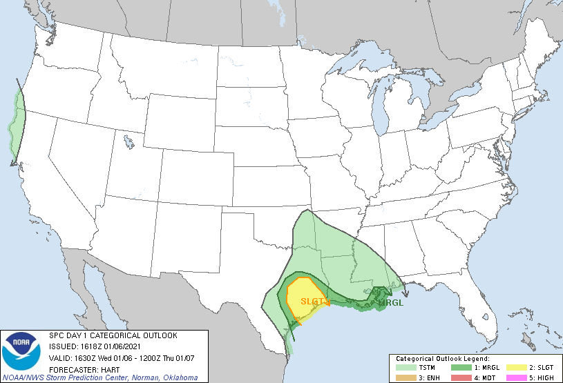
The Storm Prediction Center in Norman issued a Slight Risk (click for map, from here) of severe weather over portions of southeast TX on 6 January 2021. The Day Cloud Phase Distinction RGB, shown above (click the image to animate) shows a developing line of convection stretching through the SLGT RSK area... Read More
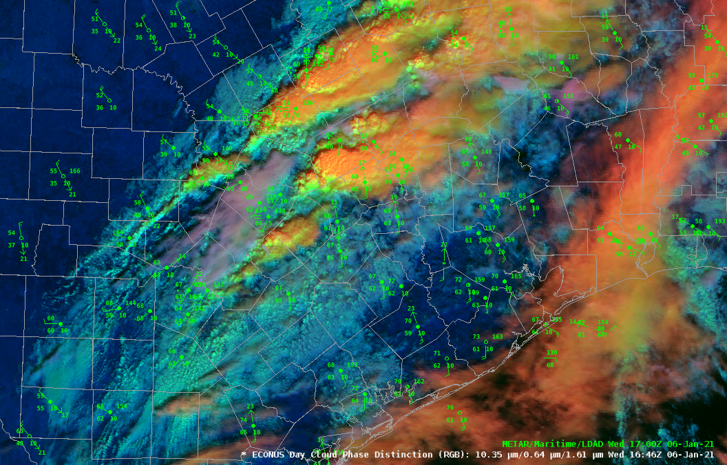
GOES-16 Day Cloud Phase Distinction RGB, 1646-2136 UTC on 6 January 2021, along with surface METARs (Click to animate)
The Storm Prediction Center in Norman issued a Slight Risk (click for map, from here) of severe weather over portions of southeast TX on 6 January 2021. The Day Cloud Phase Distinction RGB, shown above (click the image to animate) shows a developing line of convection stretching through the SLGT RSK area (The tallest convective cloud tops acquire a yellowish tint as they glaciate; lower clouds are blue/green/cyan). The Day Cloud Phase Distinction RGB also allows for easy visualization of vertical wind shear: the high cirriform clouds (orange and red) move in a distinctly different direction than the low cumuliform clouds (blue and green). A Severe Thunderstorm Watch (Watch #2 on the year) was issued at 1900 UTC (Click here for Radar image that accompanied the watch issuance). How could various satellite-based (or satellite-influenced) products be used to anticipate and to quantify the likelihood of severe weather during the day?
Polar Hyperspectral Sounding (PHS) data (from CrIS on Suomi NPP/NOAA-20 or from IASI on MetOp, for example) can augment Advanced Baseline Imager (ABI) data from GOES-16 (or GOES-17) to allow for better initialization of moisture fields in models. PHS data are linked to ABI information at the time of the polar orbiting overpass, and that relationship is carried forward in time. This data fusion process (PHSnABI) combines the excellent spectral resolution of the PHS with the superior spatial and temporal resolution of the ABI. When those data are used to initialize a model, it is frequently the case that the better moisture distribution within the PHSnABI fields leads to a more refined forecast of convection. (See this website for more information and for current model fields) Was that true on this day?
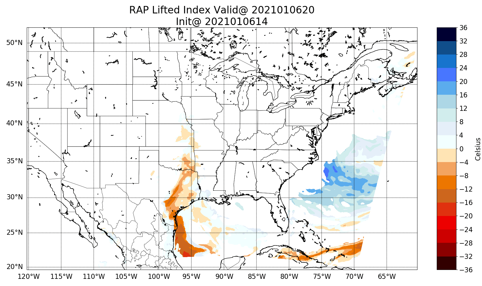
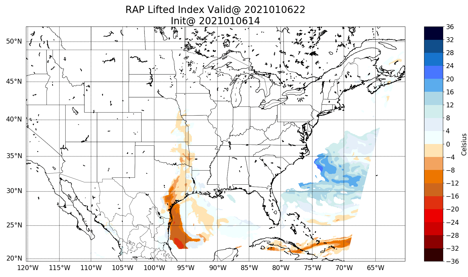
The toggles below show data from models runs initialized at 1400 and 1500 UTC, with model fields at 1800, 2000 and 2200 UTC. Lifted Index fields are shown with data from a Rapid Refresh-type simulation (that is, with no incorporation of fused PHSnABI data) identified as ‘RAP’ in the label; with data from a Single Data Assimilation (‘SDA’) system; and with data from a Continuous Data Assimilation (‘CDA’) system.
The CDA model system does appear best at simulating the timing of the convection that moves through southeast Texas (if one can use simulated Lifted Index as a proxy for the leading edge of convection).

Lifted Index at 1800 UTC from Models (RAP, SDA, and CDA) initialized at 1400 UTC (Click to enlarge)

Lifted Index at 1800 UTC from RAP, SDA and CDA models initialized at 1500 UTC (Click to enlarge)
Lifted Index at 2000 UTC from RAP, SDA and CDA models initialized at 1400 UTC (Click to enlarge)

Lifted Index at 2000 UTC from RAP, SDA and CDA models initialized at 1500 UTC (Click to enlarge)
Lifted Index at 2200 UTC from RAP, SDA and CDA models initialized at 1400 UTC (Click to enlarge)

Lifted Index at 2200 UTC from RAP, SDA and CDA models initialized at 1500 UTC (Click to enlarge)
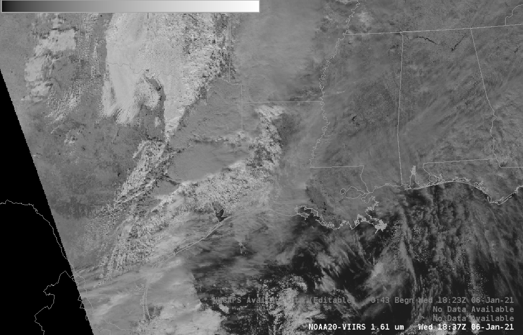
NOAA-20 VIIRS imagery at 1823 UTC: 1.61 µm, True Color and False Color (Click to enlarge)
NOAA-20 overflew the convection at 1823 UTC, and the imagery above was processed at the Direct Broadcast site at CIMSS. (It is available for AWIPS via an LDM feed, and also as imagery for one week at this website; data for other days is here). VIIRS I3 (1.61 µm), True-Color and False-Color imagery from VIIRS all show a well-developed convective system at 1823 UTC.
As the convective event is unfolding, NUCAPS profiles derived from NOAA-20 can be used to diagnose the thermodynamic state of the atmosphere. The toggle below shows 5 different profiles over southeastern Texas (along a line to the west of Galveston Bay) at ca. 1830 UTC. The green points are NUCAPS profiles for which the infrared retrieval has converged to a solution. A general decrease in stability (and increase in moisture) is apparent for profiles closer to the convection. The red point (a profile for which the infrared and microwave retrieval both failed) is included as well.

NUCAPS profiles at select points as indicated over southeast Texas, 1830 UTC on 6 January 2021 (Click to enlarge)
A simpler, faster way to view the thermodynamic fields within NUCAPS profiles is to use gridded fields. NUCAPS data are gridded onto constant pressure surfaces (using Polar2Grid software). The Total Totals Index field, below, shows a corridor of instability inland over southeast Texas with values exceeding 50.
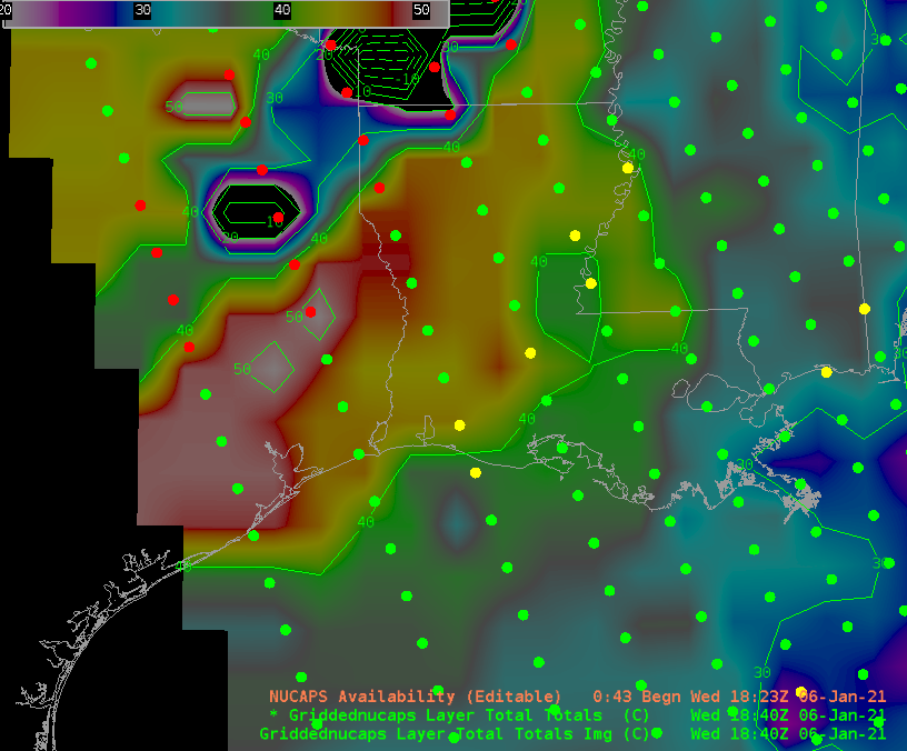
Total Totals index from gridded NOAA-20 NUCAPS values, ca. 1830 UTC (Click to enlarge)
During the actual convective outbreak, NOAA/CIMSS ProbSevere (available online here) offers a data-driven way to highlight the radar echoes most likely to be producing severe weather in the next 60 minutes. The animation below shows values at 15-minute timesteps (for simplicity); ProbSevere values can change every 2 minutes, however. Use ProbSevere in combination with radar scanning to increase confidence in warning issuance.
NOAA/CIMSS ProbSevere, every 15 minutes, 1715 – 2300 UTC on 6 January 2021 (Click to enlarge)
Severe Weather reports(source) for 6 January are shown below.

SPC Storm Reports from 6 January 2021 (Click to enlarge)
View only this post
Read Less
![GOES-16 Mid-level Water Vapor (6.9 µm) images, with hourly surface weather type plotted in yellow [click to play animation | MP4]](https://cimss.ssec.wisc.edu/satellite-blog/images/2021/01/210110_210111_goes16_waterVapor_surfaceWeather_NM_TX_LA_MS_winter_storm_anim.gif)
![GOES-16 Day Cloud Phase Distinction RGB images [click to play animation | MP4]](https://cimss.ssec.wisc.edu/satellite-blog/images/2021/01/210110_goes16_dayCloudPhaseDistinctonRGB_NM_TX_LA_winter_storm_anim.gif)
![GOES-16 Day Cloud Phase Distinction RGB and Day Snow-Fog RGB images [click to play animation | MP4]](https://cimss.ssec.wisc.edu/satellite-blog/images/2021/01/210111_goes16_dayCloudPhaseDistinctionRGB_daySnowFogRGB_NM_TX_LA_snow_cover_anim.gif)
![VIIRS True Color and False Color RGB images from Suomi NPP [click to enlarge]](https://cimss.ssec.wisc.edu/satellite-blog/images/2021/01/210111_1936utc_suomiNPP_viirs_trueColorRGB_falseColorRGB_NM_TX_snow_cover_anim.gif)


![GOES-17 "Red" Visible (0.64 µm) image, with plots of Metop-A ASCAT winds [click to enlarge]](https://cimss.ssec.wisc.edu/satellite-blog/images/2021/01/ber_vis_ascat-20210105_211031.png)
![Suomi NPP VIIRS Day/Night Band (0.7 µm) images [click to enlarge]](https://cimss.ssec.wisc.edu/satellite-blog/images/2021/01/210105_suomiNPP_viirs_dayNightBand_Bering_Sea_anim.gif)

