
GOES-16 Visible (0.64 µm) imagery and Mesoscale Sector 2 Derived Motion Winds, 1430 -1930 UTC. Winds are available every 5 minutes, imagery is also shown every 5 minutes, rather than the default 1 minute for Mesoscale Sectors (Click to animate)
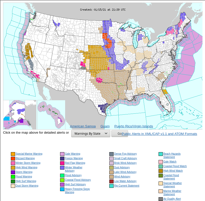
The High Plains of Kansas, Colorado, Oklahoma and Texas experienced a significant dust storm (with Dust Storm Warnings issued) on 15 January 2021, (Click here for a blog post on the blowing dust with this storm on 14 January) associated with a strong jet streak and extratropical cyclone discussed here. The animation above (Here’s the same animation, but slower) shows visible imagery along with GOES-16 Mesoscale Sector Derived Motion Winds from the Visible Channel. These derived winds are available with a 5-minute cadence, and the dust was thick enough that features could be tracked. There aren’t a lot of derived winds; how well do these derived winds compare to surface winds?
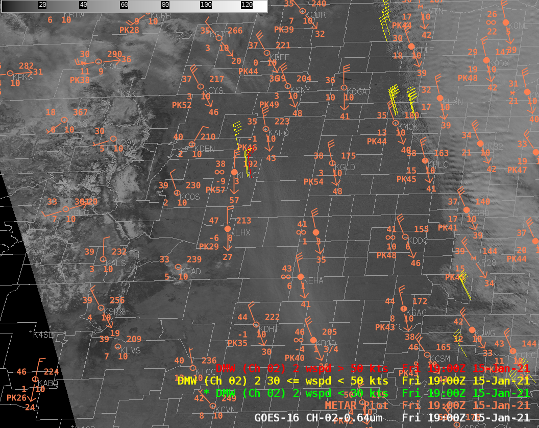
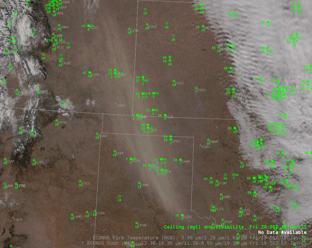
METAR Observations, GOES-16 Visible (0.64 µm) imagery, and Derived Motion Winds from Visible data, 1900 UTC on 15 January 2021 (Click to enlarge)
The image above, from 1900 UTC, shows Derived Motion winds along with METAR observations. Derived Motion winds are stronger than surface winds, as expected; compare, for example, the observations at Limon CO (KLIC) with the nearby derived wind vectors. The levels of the derived motion winds are between 800-820 hPa, away from the effects of friction/surface roughness. However, they do give a nice estimate of what surface winds might be in regions without surface observations, as apparent in the animation at the top.
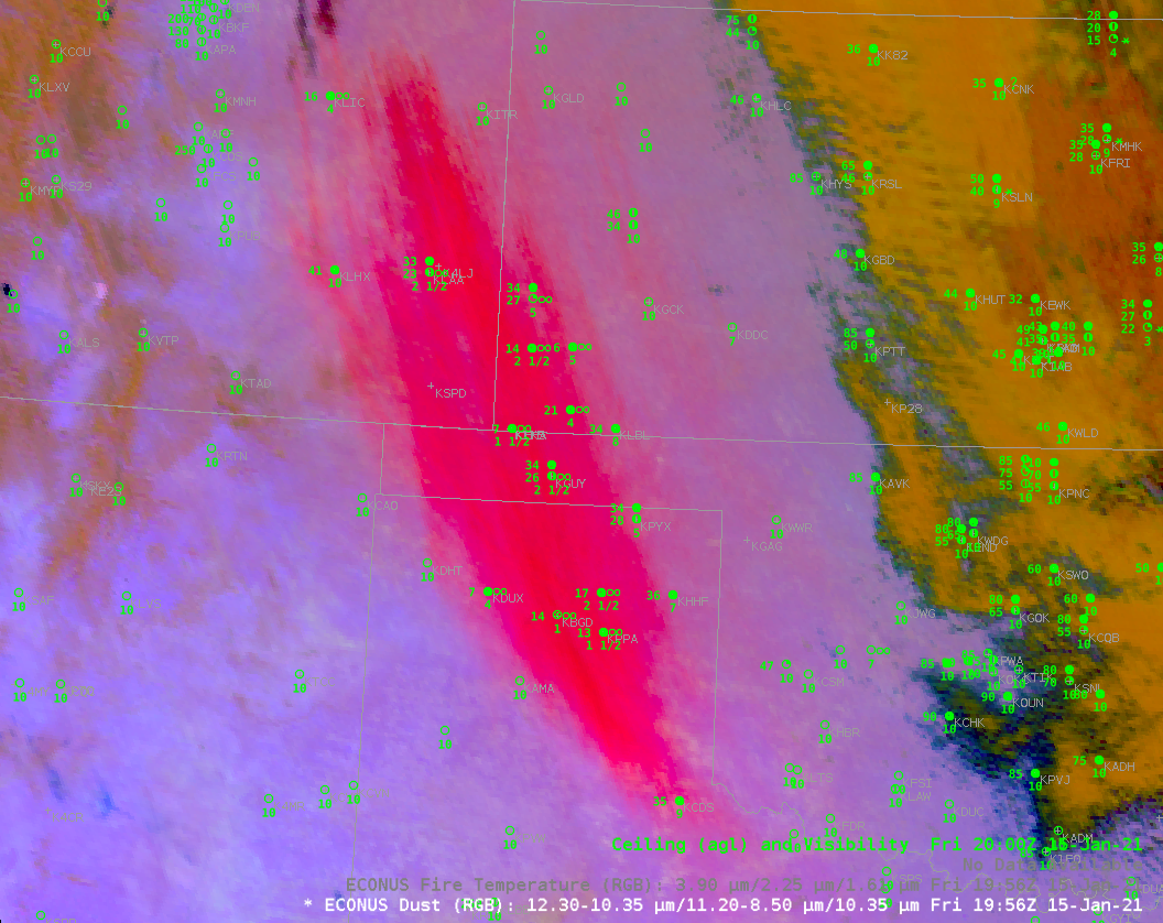
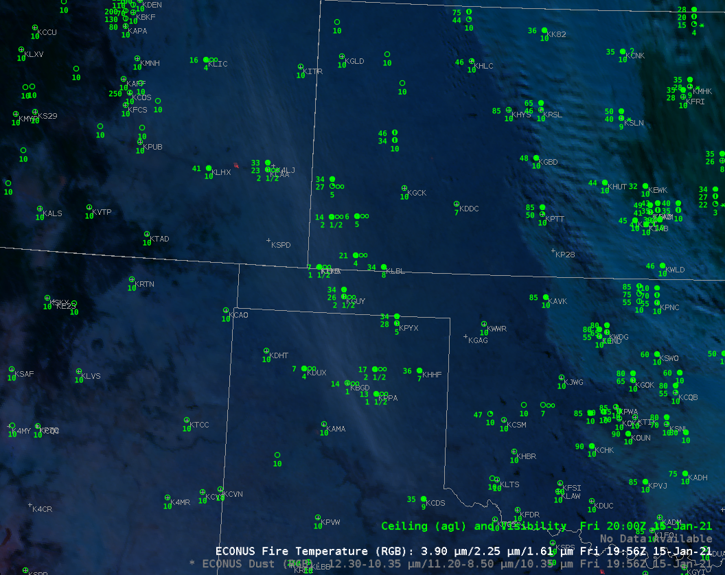
It can be difficult to view dust with just one ABI channel such as the visible, especially when the sun is high(ish) in the sky and there is little forward scattering. Multi-spectral RGB products, such as the GOES-16 Dust RGB, shown below in a toggle with a VIIRS True-Color image and the GOES-16 Fire RGB (there is a fire evident near KLHX, LaJunta, CO), are a valuable tool in identifying the horizontal extent of dust plumes. Dust is highlighted in the Dust RGB by a vivid pink/magenta color.
NOAA-20 VIIRS True-Color image, GOES-16 Dust RGB and GOES-16 Fire Temperature RGB at 1956 UTC, 15 January 2021 (Click to enlarge)
View only this post Read Less
![GOES-16 Upper-level Water Vapor (6.2 µm) images, with plots of hourly surface wind barbs and gusts [click to play animation | MP4]](https://cimss.ssec.wisc.edu/satellite-blog/images/2021/01/210114_goes16_waterVapor8_surfaceWinds_Plains_anim.gif)
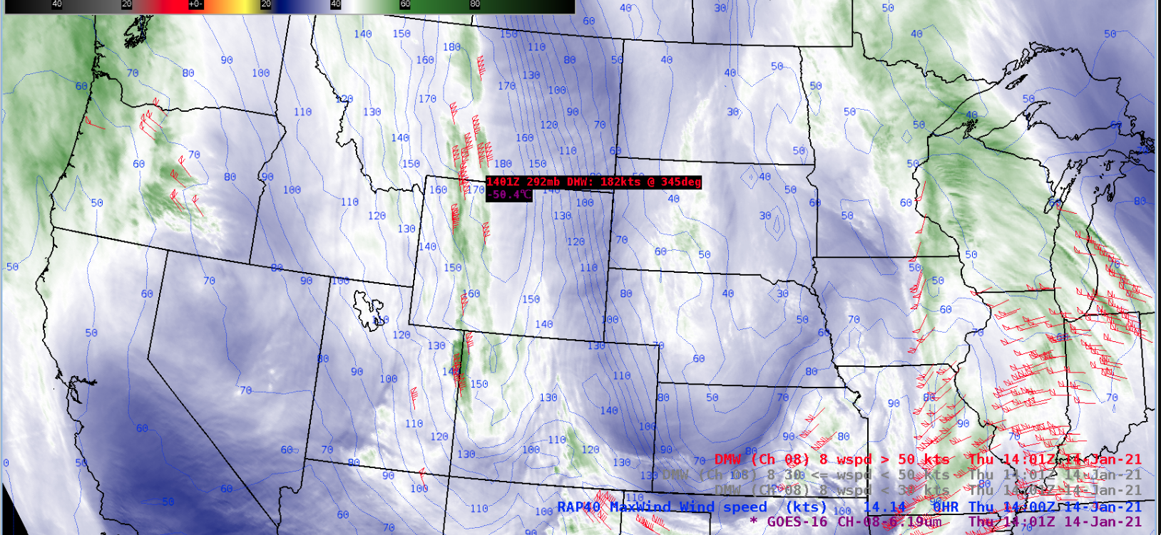
![GOES-16 Upper-level Water Vapor (6.2 µm) images, with plots of 6.2 µm Derived Motion Winds and contours of RAP40 model maximum wind speeds [click to play animation | MP4]](https://cimss.ssec.wisc.edu/satellite-blog/images/2021/01/210114_goes16_waterVapor_derivedMotionWinds_Rockies_jet_anim.gif)
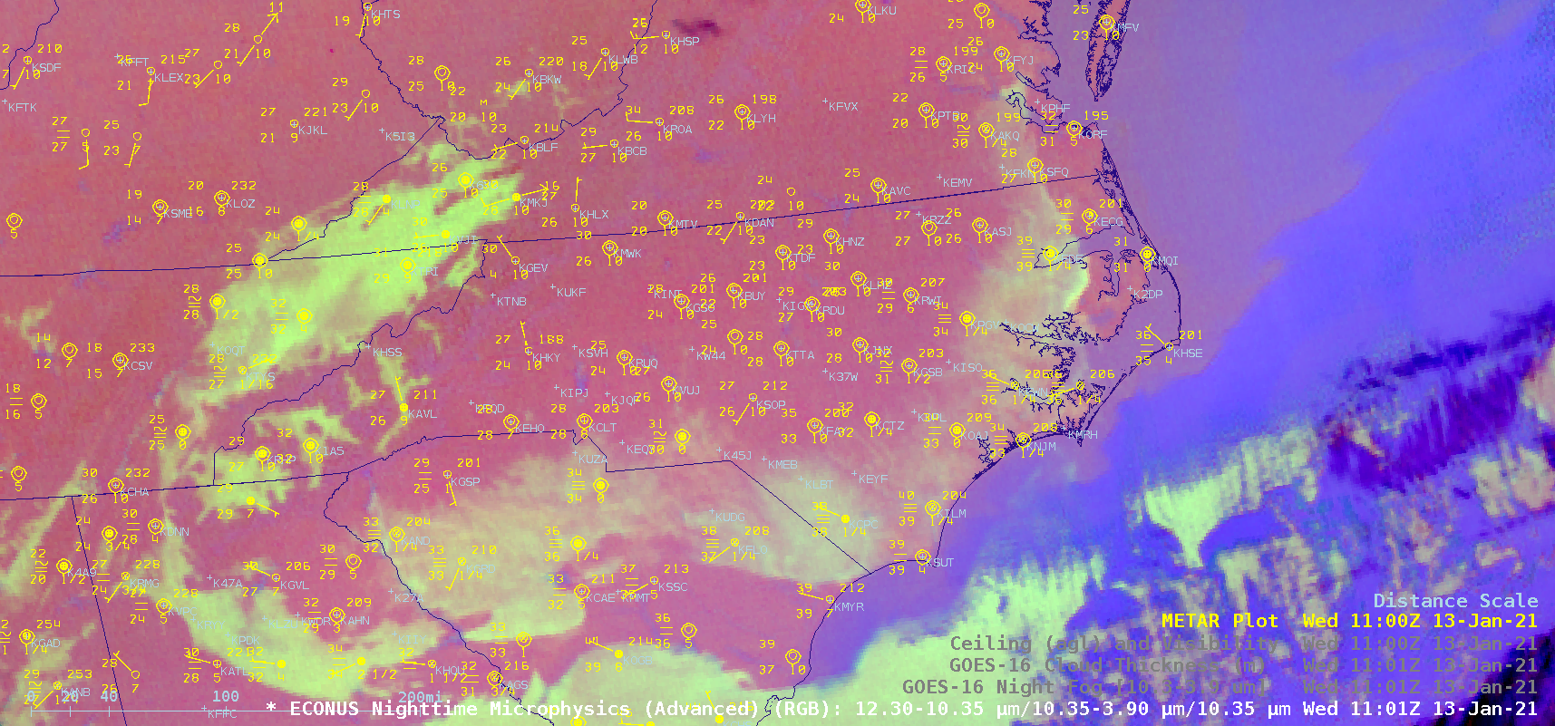
![GOES-16 Nighttme Microphysics, Night Fog BTD (10.3-3.9 µm) and Cloud Thickness product [click to play animation | MP4]](https://cimss.ssec.wisc.edu/satellite-blog/images/2021/01/210113_goes16_nighttimeMicrophysicsRGB_nightFogBTD_cloudThickness_SC_NC_VA_freezing_fog_anim.gif)
![GOES-16 Nighttime Microphysics RGB images, with plots of surface observations [click to play animation | MP4]](https://cimss.ssec.wisc.edu/satellite-blog/images/2021/01/210113_goes16_nighttimeMicrophysicsRGB_surfaceObservations_SC_NC_VA_freezing_fog_anim.gif)
![GOES-16 Nighttime Microphysics RGB image, with a plot of NAM40 model 925 hPa winds at 12 UTC [click to enlarge]](https://cimss.ssec.wisc.edu/satellite-blog/images/2021/01/nc_ntm_925winds-20210113_120115.png)

