This website works best with a newer web browser such as Chrome, Firefox, Safari or Microsoft
Edge. Internet Explorer is not supported by this website.
Scientists at STC and at SPoRT have created a website to view NUCAPS profiles using Sharppy and cloud resources. The animation above shows the user interface for Observed Soundings (i.e., upper-air soundings), for NUCAPS Soundings for different passes, and NAM Nest model profiles. The green points have been chosen for... Read More
Available soundings from divers sources between 0000 and 1200 UTC on 29 September over the United States (Click to enlarge)
Scientists at STC and at SPoRT have created a website to view NUCAPS profiles using Sharppy and cloud resources. The animation above shows the user interface for Observed Soundings (i.e., upper-air soundings), for NUCAPS Soundings for different passes, and NAM Nest model profiles. The green points have been chosen for subsequent display. Points near KARB — Aberdeen, South Dakota — were selected; on this day, subsequent NOAA-20 NUCAPS passes produced data 90 minutes apart very near Aberdeen.
Soundings in/around Aberdeen SD: 0000 UTC Radiosonde, 0735 UTC NOAA-20 NUCAPS Sounding, 3-h Forecast soundings from the NAM Nest, valid at 0900 UTC, 0915 UTC NOAA-20 NUCAPS Sounding, 1200 UTC Radiosonde; the final image includes all the soundings at once (Click to enlarge)
The toggle between the 0000 and 1200 UTC radiosondes at Aberdeen shows a general moistening of the atmosphere (especially above 500 mb). NUCAPS soundings in between give a forecaster information on the character of that increase: linear? step-wise? The two NUCAPS soundings, below, separated by 90 minutes, and in between the two radiosondes, show moistening after 0700 UTC.
NOAA-20 NUCAPS Soundings near Aberdeen, SD, 0745 and 0915 UTC on 29 September 2021 (Click to enlarge)
NUCAPS soundings are volumetric, in comparison the radiosonde and model-derived soundings, both of which are valid at one point that is ascending through the atmosphere. NUCAPS soundings from NOAA-20 are a blend of information from up to 9 CrIS (Cross-track Infrared Sounder) fields of regard and one Advanced Technology Microwave Sounder (ATMS) footprint. A comparison between radiosonde or model soundings and NUCAPS soundings should always be tempered with that information.
Fires burning in far northern Paraguay on 29 September 2021 created a pyrocumulonimbus or pyroCb cloud — GOES-16 (GOES-East) “Red” Visible (0.64 µm), Shortwave Infrared (3.9 µm) and “Clean” Infrared Window (10.35 µm) images (above) showed the pyroCB cloud, fire thermal anomalies or “hot spots” (clusters of red pixels) and cold cloud-top infrared brightness temperatures, respectively.... Read More
GOES-16 Visible (0.64 µm, top), Shortwave Infrared (3.9 µm, center) and Infrared Window (10.35 µm, bottom) images [click to play animation | MP4]
Fires burning in far northern Paraguay on 29 September 2021 created a pyrocumulonimbus or pyroCb cloud — GOES-16 (GOES-East) “Red” Visible (0.64 µm), Shortwave Infrared (3.9 µm) and “Clean” Infrared Window (10.35 µm) images (above) showed the pyroCB cloud, fire thermal anomalies or “hot spots” (clusters of red pixels) and cold cloud-top infrared brightness temperatures, respectively. The minimum 10.35 µm temperature was -47.6ºC at 1840 UTC. Note the relatively warm (darker gray) appearance of the pyroCb cloud in the 3.9 µm images — this is a characteristic signature of pyroCb cloud tops, driven by the smoke-induced shift toward smaller ice particles (which act as more efficient reflectors of incoming solar radiation).
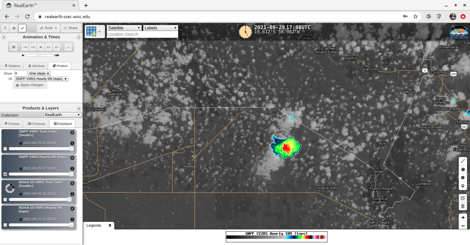
A Suomi-NPP VIIRS Infrared Window (11.45 µm) image at 1751 UTC as viewed using RealEarth(below) revealed cloud-top infrared brightness temperatures in the -60s C (shades of red). Surface temperatures at nearby sites had reached 38ºC (100ºF) by 18 UTC.
Suomi-NPP VIIRS Infrared Window (11.45 µm) image at 1751 UTC [click to enlarge]
South American pyrocumulonimbus clouds are fairly uncommon — since the first documented case in 2018, only 7 other pyroCbs have been identified over that continent.
Thanks to Mike Fromm, NRL, for alerting us to this latest pyroCb case. Additional information is available from Metsul.com.
According to the JPL site, there was a bright meteor (or bolide) on September 29, 2021 over the Gulf of Alaska. (The JPL and a similar NASA site are posted under the GLM tab on this link of links.) This event was seen by both the ABI and GLM on NOAA‘s GOES-17, as well as the... Read More
According to the JPL site, there was a bright meteor (or bolide) on September 29, 2021 over the Gulf of Alaska. (The JPL and a similar NASA site are posted under the GLM tab on this link of links.) This event was seen by both the ABI and GLM on NOAA‘s GOES-17, as well as the AHI on Japan’s Himawari-8. What may be unique about his event is that the imagers monitored the meteor soon after it’s explosion, and not just the resulting plume (as was done in this case over Russia in 2013). This is based on the length of the event, during which the various spectral bands displayed a signature and other information.
Peak Brightness Date
Peak Brightness Time (UT)
Latitude (deg.)
Longitude (deg.)
Altitude (km)
Total Radiated Energy (J)
Calculated Total Impact Energy (kt)
2021-09-29
10:50:59
53.9N
148.0W
28
13.7e10
0.4
Entry from table via the JPL site.
GOES-17
The GLM and ABI observed this event, but given it’s faster readout, the GLM offers much more information than the ABI. The apparent location of the meteor as seen by the ABI is different than the reported location, in part due to parallax. More on the concept of parallax is available here.
Animation of GOES-17 ABI band 12 (9.6 mirometer) mesoscale sector #2 on September 29, 2021.
Hotter brightness temperatures can be seen in the GOES-17 ABI band 12 at 10:50:59 UTC.
Animation of all 16 bands of the GOES-17 imager on September 29, 2021. Note band 12.
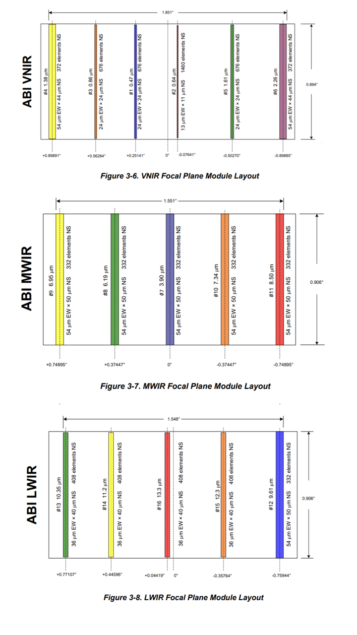
Indicative of a short duration event, coupled with how the ABI scans, the meteor signature was only clearly seen at one time in nearly every ABI spectral band (although possibly the ABI band 11 as well). Due to the layout of the focal plane array on the ABI, not all spectral bands observe the Earth at the precisely same time. [Figure a modification from the GOES-R Series Data Book.] A similar loop as above, but as an animated gif, is available here. In addition,. while a bit hard to see, the longwave split window infrared difference also showed a subtle signature of the meteor.
Spectral difference images (over time) can also be useful in the monitoring of meteors. An ABI 10.3 – 12.3 micrometer band difference is shown below. An shortwave minus longwave difference loop.
An animation of the GOES-17 difference image between ABI 10.3 – 12.3 micrometer bands. The brightness temperature range is -5 to +5K.
The GLM on GOES-17 also observed this event. A similar loop as below, but as an animated gif, is available.
ABI band 12 and the GLM Flash Event Group density on September 29, 2021. Credit: CIRA/RAMMB Slider.
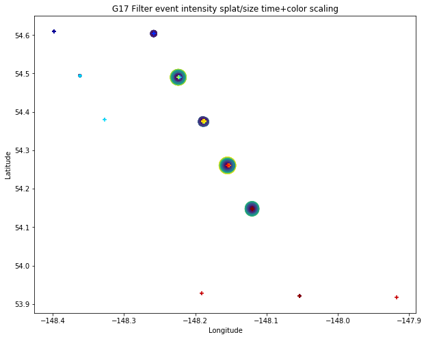
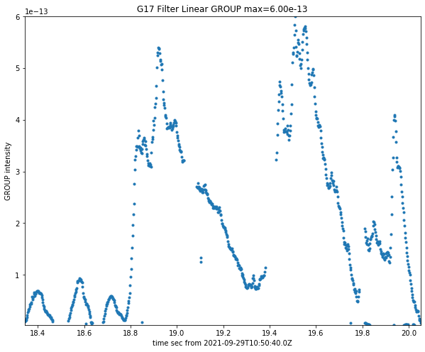
The rapid movement of the meteor to the south is clearly evident. As well as the GLM group map and the key (blue is early times and red is later times).
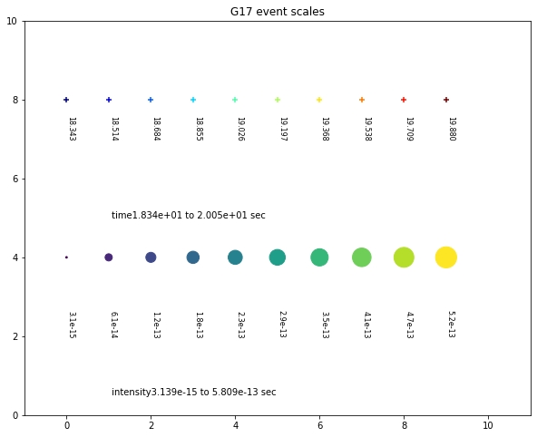
GOES-17 GLM meteor location over time and space on September 29, 2021 with larger circles (color coded to intensity). Credit: Todd Beltracchi.
As well as the changes over time, most likely monitoring the meteor break-ups.
GOES-17 GLM meteor over time on September 29, 2021. Credit: Todd Beltracchi.
Both the ABI and Japan’s AHI scan space around the edge of the Earth. However, with the ABI data the process of making calibrated, navigated, and remapped radiance only pixels located on the Earth are included in the Level 1b radiance files. Hence, the ABI may scan meteors in space, but the data are not available to most users.
All 16 spectral bands from Himawari-8 AHI at the same nominal time (10:50 UTC) on September 29, 2021.
A similar loop as above, but as an animated gif, is available here (and an 8-panel AHI image at this same time is available here). This example helps to illustrate that each AHI detector doesn’t sense radiation from the same exact location at the same time.
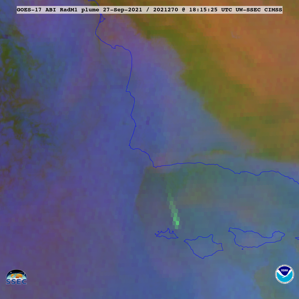
The ABI on NOAA‘s GOES-17 (GOES-West) was able to see the Landsat 9 rocket plume from Vandenberg Space Force base. The plume was most evident on ABI bands 7 (3.9 µm) and 8 (6.2 µm), using the mesoscale sector (1) on September 27, 2021.
The 16 spectral bands from GOES-17 on September 27, 2021 off the coast of California. Note bands 7 and 8.


