EUMETSAT Meteosat-9 Infrared Window (10.8 µm) images (above) showed Cyclone Hidaya as it intensified from a Tropical Storm (at 1200 UTC on 02 May) to Category 1 Hurricane intensity at 0000 UTC on 03 May 2024 (advisory | discussion). JTWC later noted that Hidaya had become the most intense tropical... Read More

EUMETSAT Meteosat-9 Infrared Window (10.8 µm) images, from 1200 UTC on 02 May to 1200 UTC on 03 May [click to play animated GIF | MP4]
Meteosat-9 Infrared Window (10.8 µm) images
(above) showed Cyclone Hidaya as it intensified from a Tropical Storm (at 1200 UTC on 02 May) to Category 1 Hurricane intensity at 0000 UTC on 03 May 2024 (
advisory |
discussion).
JTWC later noted that Hidaya had become the most intense tropical cyclone on record for this region, peaking at 80 kt (
discussion).
A DMSP-18 SSMIS Microwave (85 GHz) image at 0024 UTC on 03 May, from the CIMSS Tropical Cyclones site (below) revealed a well-defined eye and surrounding eyewall structure.
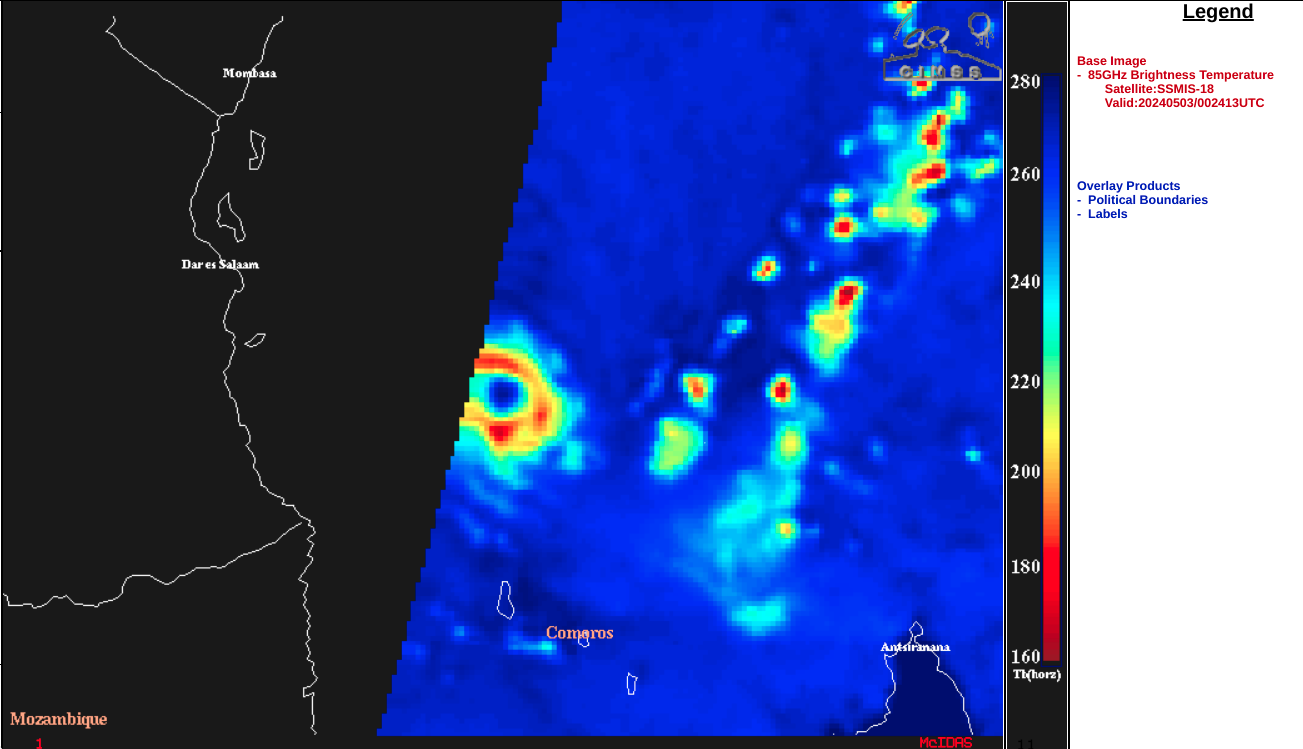
DMSP-18 SSMIS Microwave (85 GHz) image at 0024 UTC on 03 May [click to enlarge]
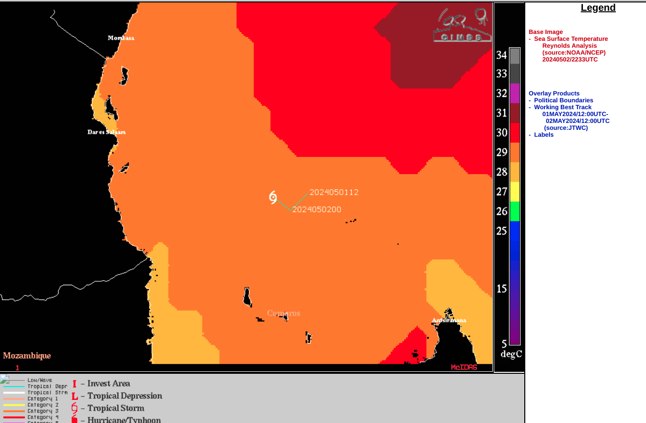
Cyclone Hidaya had been moving across
warm water and through an environment of fairly low
deep-layer wind shear (below), two factors which were favorable for intensification.
Meteosat-9 Infrared Window images, with contours and streamlines of deep-layer wind shear at 0000 UTC on 03 May [click to enlarge]
An overpass of RCM-3 provided Synthetic Aperture Radar (SAR) imagery (
source) at 1531 UTC on 02 May
(below) — the maximum sensed wind speed was 74.94 kt in the SE quadrant of the eyewall.
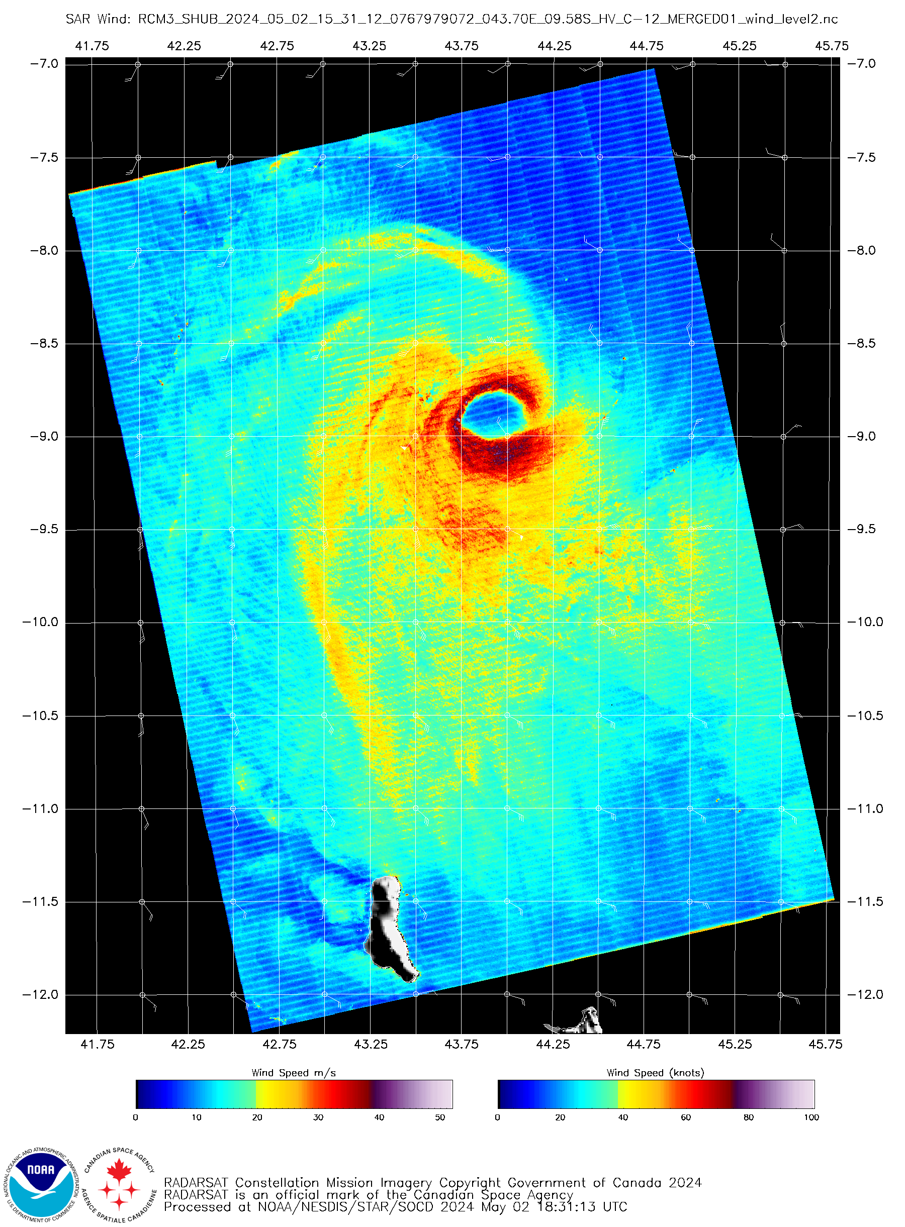
RCM-3 SAR image at 1531 UTC on 02 May [click to enlarge]
However, an overpass of RCM-3 at 1539 UTC on 03 May
(below) sensed a maximum velocity of 92.29 kt in the NE quadrant.
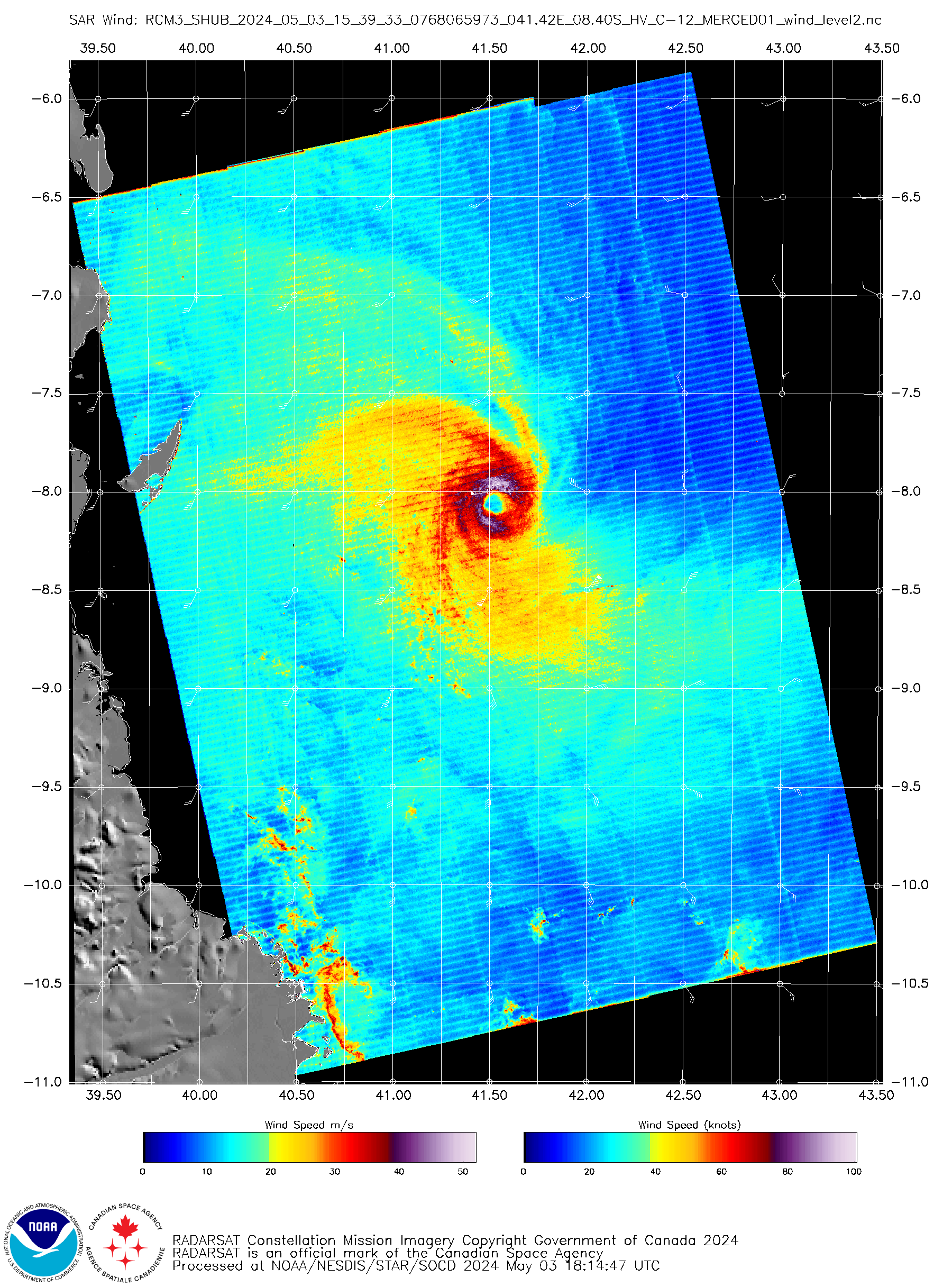
RCM-3 SAR image at 1539 UTC on 03 May [click to enlarge]
===== 04 May Update =====
EUMETSAT Meteosat-9 Infrared Window (10.8 µm) images, from 1200 UTC on 03 May to 1200 UTC on 04 May [click to play animated GIF | MP4]
Although Hidaya weakened to Tropical Storm intensity at 0000 UTC on 04 May (
track), Meteosat-9 Infrared images
(above) showed that a few brief convective bursts occurred as the tropical cyclone was approaching the coast of Tanzania. Hidaya made landfall by about 0300 UTC on 04 May (near Mafia Island), while still at Tropical Storm intensity.
View only this post
Read Less


