
GOES-13 0.63 µm visible images
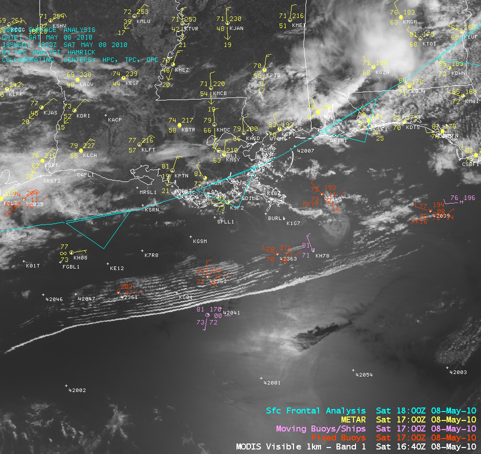
McIDAS images of GOES-13 0.63 µm visible channel data (above) revealed the formation of a packet of wave clouds over the northern Gulf of Mexico, associated with an undular bore moving southward ahead of an advancing cold frontal boundary on 08 May 2010.
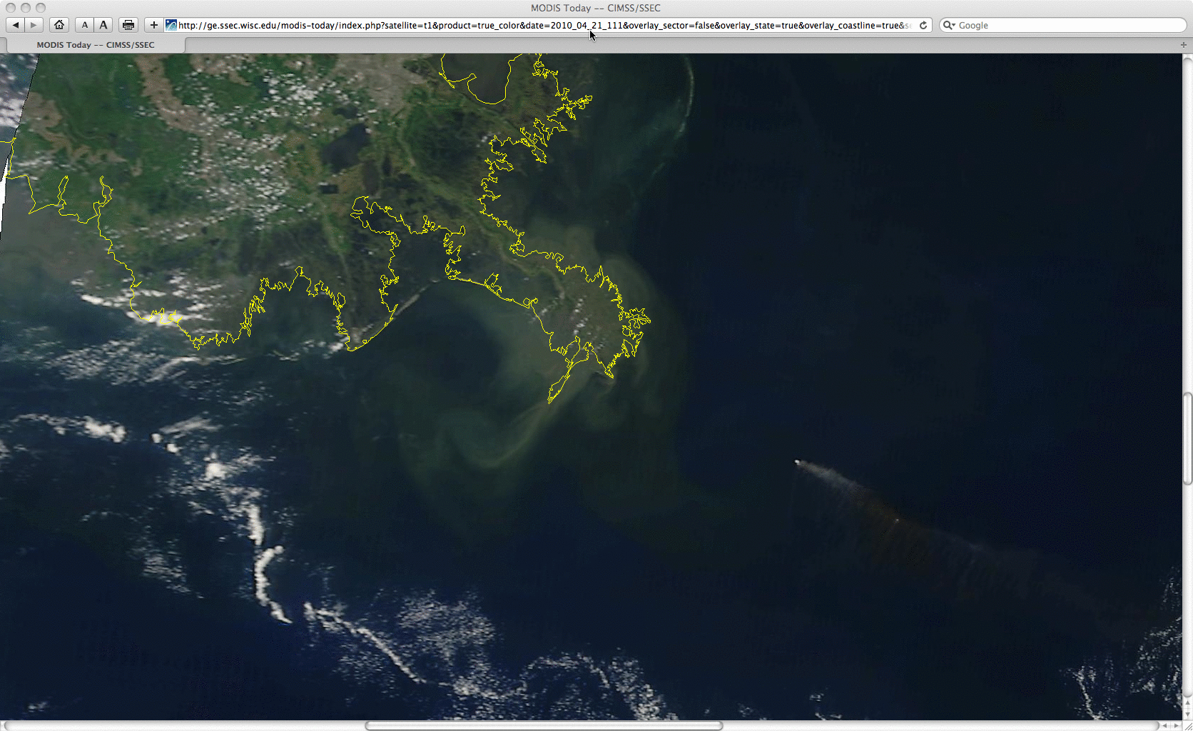
The clouds eventually cleared out enough to reveal portions of the oil slick (which remained off the coast of Louisiana following from the explosion and sinking of the Deepwater Horizon offshore oil rig) on 250-meter resolution Red/Green/Blue (RGB) MODIS true color and false color images sourced from the SSEC MODIS Today site (below). Since the oil slick feature was once again located within the sun glint portion of the MODIS image swath, it was very easy to detect on the true color (created using bands 1/4/3 as the R/G/B channels) and false color (created using bands 7/2/1 as the R/G/B channels) imagery.
It appears as though a thin filament of the oil slick has recently been drawn westward (away from the core area of the oil slick near the source), and has been entrained into the sediment outflow region of the Mississippi River. You can follow the changes in appearance of the oil slick on this comparison of MODIS true color image from 21, 25, and 29 April and 01, 04, and 08 May.
 and false color (bands 7/2/1) images")
MODIS true color (bands 1/4/3) and false color (bands 7/2/1) images
The oil slick appears as a light gray feature on an AWIPS image of the MODIS 0.65 µm visible channel data, but shows up as a very warm (darker gray to black enhancement) area on the MODIS 3.7 µm “shortwave IR” image due to a high amount of sun glint reflection of solar radiation off the oil slick surface. However, note that the oil slick feature does not exhibit any sort of signature at all on the MODIS 11.0 µm “IR window” image (below).

MODIS 0.65 µm visible, 3.7 µm
===== 09 MAY UPDATE =====
 and false color (bands 7/2/1) Red/Green/Blue (RGB) images")
MODIS true color (bands 1/4/3) and false color (bands 7/2/1) Red/Green/Blue (RGB) images
The oil slick was once again a very obvious feature in the 250-meter resolution MODIS true color and false color images on 09 May 2010 (above). In this case, note the appearance of the light pink colored pixel near the center of the oil slick on the false color image — the near-IR Band 7 used in that particular RGB image is also sensitive to hot surfaces (for example, due to a fire), which would make such a feature show up as a light pink feature. Indeed, an AWIPS image of the MODIS 3.7 µm shortwave IR channel data (below) confirmed the presence of a relatively hot pixel (43.5º C, orange color enhancement), which could have been due to a small spot fire that was set in an attempt to burn off some of the surface oil.

MODIS 0.65 µm visible and 3.7 µm shortwave IR images
===== 10 MAY UPDATE =====
 and false color (bands 7/2/1) images")
MODIS true color (bands 1/4/3) and false color (bands 7/2/1) images
The oil slick was once again a prominent feature in the 250-meter resolution MODIS true color and false color images on 10 May 2010 (above). However, note that the appearance of the oil slick was a bit different than what was seen on the previous days when sun glint was helping to illuminate the feature: on this particular day, the “brighter” portion of the oil slick appeared to be surrounded by a very dark signature. It is not entirely clear what this “dark signature” was on the MODIS true color imagery — but one idea is that it could have been due to oil that was still sub-surface (and had not yet come to the surface where it could then help to reflect light back up toward the satellite in the sun glint region of the overpass swath).
View only this post Read Less

")
")


")

