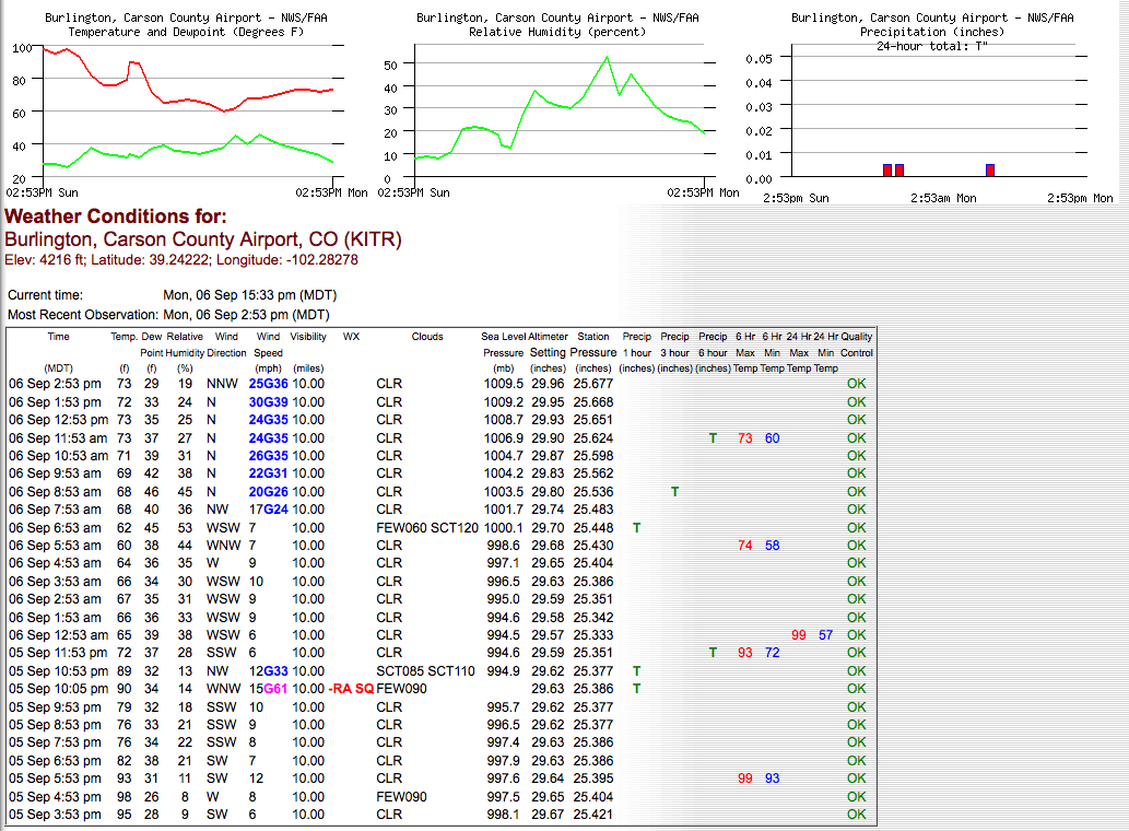
This website works best with a newer web browser such as Chrome, Firefox, Safari or Microsoft Edge. Internet Explorer is not supported by this website.

Tornado outbreak in Texas and Oklahoma

The first tornado-related fatalities of the 2009 severe weather season occurred during a tornado outbreak that affected parts of Texas and Oklahoma (SPC storm reports) on 10 FebruaryRead More

GOES-12 10.7 µm IR images

GOES-12 10.7 µm IR images

The first tornado-related fatalities of the 2009 severe weather season occurred during a tornado outbreak that affected parts of Texas and Oklahoma (SPC storm reports) on 10 February11 February 2009. GOES-12 10.7 µm IR images (above; QuickTime animation) showed the development of multiple lines of severe convection during the afternoon and evening hours of 10 February, with large areas of cloud top temperatures in the -55º to -65º C range (orange to darker red color enhancement).

The tornado fatalities occurred in the town of Lone Grove  — located just west of Ardmore in far southern Oklahoma — around 01:30 UTC (7:30 pm local time). A comparison of GOES-11, GOES-12, and GOES-13 IR images around that time (below) demonstrated the effect of “parallax”, which leads to the apparent displacement of the cold “overshooting top”  cloud feature due to varying satellite view angles. Using GOES-11 (positioned over the Pacific Ocean at 135º West longitude), the coldest overshooting top IR pixel (with an IR brightness temperature of -63º C, darker red color enhancement) was located about 5 km southeast of Ardmore (KADM). Using GOES-12 (positioned over the Atlantic Ocean at 75º West longitude), the coldest IR pixel (also -63º C) was located about 22 km west of Ardmore. Finally, the GOES-13 satellite (positioned at 105º West longitude) had a more direct viewing angle, and therefore less of a parallax error: the coldest IR pixel (-64º C) was located 12 km northwest of Ardmore — this places the “overshooting top” a few km to the north of Lone Grove, which would be the expected location.

GOES-11, GOES-12, and GOES-13 10.7 µm IR images

GOES-11, GOES-12, and GOES-13 10.7 µm IR images

A closer view using the GOES-12 visible channel images (below; QuickTime animation) shows the development of the initial line of storms over Oklahoma. The storm that produced the fatal tornado at Lone Grove formed  to the east of the main line of storms, and began to appear  just south of the Oklahoma/Texas border near the end of the animation.

GOES-12 visible images

GOES-12 visible images

AWIPS images of the GOES sounder Lifted Index (LI) derived product (below) showed that the atmosphere was destabilizing during the afternoon hour, with LI values over Oklahoma as low as -8º C by 19:00 UTC and -13º C by 21:00 UTC.

GOES-12 sounder Lifted Index derived product images

GOES sounder Lifted Index derived product images

In addition, the GOES sounder Total Precipitable Water (TPW) derived product images (below) indicated  that there was a northward surge of moisture across Oklahoma during the hours leading up to convective development, with TPW values  exceeding 20 mm (0.8 inch) by 18:00 UTC, and TPW values exceeding 30 mm (1.2 inches) by 21:00 UTC.

GOES-12 sounder Total Precipitable Water derived product images

GOES sounder Total Precipitable Water derived product images

A strong upper-level trough was moving eastward across the southern Rocky Mountains region, and the GOES sounder Total Column Ozone derived product images (below) depicted elevated values of ozone associated with this trough. Total Column Ozone values of 350-425 Dobson Units (green to red color enhancement) often correspond to a lowering of the dynamic tropopause and/or the presence of a potenial vorticity (PV) anomaly — and the approach of the trough and the associated PV anomaly likely helped to produce an environment that favored  upward vertical motions on a synoptic scale across the southern Plains region late in the day on 10 February.

GOES-12 sounder Total Column Ozone derived product images

GOES sounder Total Column Ozone derived product images

View only this post Read Less

Melting snow and thinning ice

The National Weather Service at Milwaukee/Sullivan posted a nice animation of MODIS true color imagery (using the  AWIPS “MODIS True Color Imagery Viewer” that Jordan Gerth developed as part of the CIMSS/SSEC Read More

MODIS true color and false color images

MODIS true color and false color images

The National Weather Service at Milwaukee/Sullivan posted a nice animation of MODIS true color imagery (using the  AWIPS “MODIS True Color Imagery Viewer” that Jordan Gerth developed as part of the CIMSS/SSEC MODIS in D2D project) which shows the breakup of ice in southern Lake Michigan and the melting of snow cover over far southeastern Wisconsin during a 3-day period of warm temperatures in early February 2009. A comparison of MODIS “true color” (Red/Green/Blue composite using channels 01/04/03) and “false color” (Red/Green/Blue composite using channels 07/02/01) images from the SSEC MODIS Today site (above) also showed some interesting clues about the thinning of the ice on some of the inland lakes and rivers on 08 February 2008. Snow and ice appear as white features on the true color image, but appear as varying shades of cyan on the false color image — however, thinner ice shows up as a darker blue color on the false color image (due in part to a higher meltwater content within  the top layer of the ice).

Even though the appearance of the inland lake ice was beginning to show signs of degradation and thinning  on the MODIS imagery, recent reports of ice thickness (below, courtesy of Lake-Link.com) indicated that there was still over 20 inches of ice on some parts of the larger lakes such as Lake Winnebago (the largest lake in east-central Wisconsin), as well as on smaller lakes like Lake Mendota (the largest of the lakes in the Madison area). Note that some of the lakes in southern Wisconsin are already ice-free — these lakes exhibit a darker appearance on both the true color and the false color images. In addition, a significant amount of lake ice can still be seen along the eastern nearshore waters of Lake Michigan.

Lake Winnebago ice thickness

Lake Winnebago ice thickness (courtesy of Lake-Link.com)

Lake Mendota ice thickness

Lake Mendota ice thickness (courtesy of Lake-Link.com)

View only this post Read Less

Of lake-effect snow bands, ice floes, and satellite navigation

A side-by-side comparison of GOES-12 and GOES-13 visible images (above) shows a well-defined lake-effect cloud band that was oriented generally north-to-south across Lake Michigan on 04 February 2009. This narrow cloud band was producing heavy snow as it moved inland over far... Read More

GOES-12 and GOES-13 visible images

GOES-12 (left) and GOES-13 (right) visible images

A side-by-side comparison of GOES-12 and GOES-13 visible images (above) shows a well-defined lake-effect cloud band that was oriented generally north-to-south across Lake Michigan on 04 February 2009. This narrow cloud band was producing heavy snow as it moved inland over far northwestern Indiana, with 15-20 inches of storm total accumulation reported. The GOES-12 and GOES-13 images are displayed in their native satellite projections (GOES-12 is positioned over the Equator at 75º West longitude, while GOES-13 is positioned at 105º West longitude).

The improved Image Navigation and Registration (INR)  system on the GOES-13 satellite is immediately obvious, with much less image-to-image “wobble” — and the better navigation of the GOES-13 imagery makes it easier to follow the motion of the ice floes that were drifting over both the western and eastern nearshore waters of Lake Michigan.

Even with the GOES-12 images being re-mapped for display in AWIPS (below), the amount of image-to-image wobble is still obvious. Hourly MADIS winds (or “atmospheric motion vectors”) are also plotted on the visible imagery — these winds are derived by following targets on 3 consecutive satellite images.

GOES-12 visible images

AWIPS GOES-12 visible images

A closer view of southern Lake Michigan using 250-meter resolution MODIS true color images from the SSEC MODIS Today site (below) suggests that the ice along the eastern nearshore waters is probably thicker (and likely snow-covered as well).

MODIS true color images

MODIS true color images

Farther to the north, cold temperatures over the northern Great Lakes region (the morning low on 04 February was -36º F or -38º C at Babbit in northeastern Minnesota, and -28º  F or -33º C at Minong in northwestern Wisconsin) led to increased ice coverage over Lake Superior, as seen in 250-meter resolution MODIS false color imagery from the Terra and Aqua satellites (below). The ice in the lake appears as cyan-colored features, in contrast to supercooled water droplet clouds (which appear as varying shades of white). Note that there are more lake-effect cloud bands over the eastern portion of Lake Superior, where there is much less ice coverage — the ice covering much of the western portion of the lake reduces the amount of heat flux necessary to form the lake-effect cloud bands.

MODIS false color images

MODIS false color images

Speaking of lakes and their effect on cloud bands and snowfall, there was also an interesting case of “lake-enhanced” snow on this particular day, immediately downwind of Lake Marion and Lake Moultrie in South Carolina (hat-tip to Jon Jelsema at NWS Charleston SC for bringing this to our attention). A MODIS true color image (below, viewed using Google Earth) showed the cluster of cloud bands that were streaming southeastward from the 2 lakes, producing moderate to heavy snow that was reducing visibility as low as 1/4 mile.

MODIS true color image (viewed using Google Earth)

MODIS true color image (viewed using Google Earth)

It is interesting to note that a small patch of “transverse band” clouds formed for a brief time, apparently at a slightly higher altitude than the lake-enhanced cloud bands — these transverse bands were more obvious on a NOAA-17 “false color” red/green/blue (RGB) image (below). An animation of GOES-13 visible imagery shows the development of the lake-enhanced cloud bands and the higher-altitude transverse bands — they are both very subtle and appear only briefly, but they are there if you look closely!

NOAA-17 false color RGB image

NOAA-17 false color RGB image

— 05 FEBRUARY UPDATE —

The surface winds shifted from northerly on 04 February to southerly on 05 February,  which caused the ice that was floating in the nearshore areas of  Lake Michigan to begin drifting northward during the day. This northward drift was clearly seen on GOES-12 and GOES-13 visible imagery (below). You can even see that the “land-fast” ice at the extreme southern end of the lake appeared to break free during the afternoon hours.

GOES-12 (left) and GOES-13 (right) visible images

GOES-12 (left) and GOES-13 (right) visible images

View only this post Read Less

Ice storm over the south-central US

MODIS visible + snow/ice images AWIPS images of the MODIS visible channel and the 2.1 µm near-IR “snow/ice discrimination” channel (above) showed the areal coverage of surface snowfall and ice accrual across much of the southern Plains on 28 January 2009. Many... Read More

MODIS visible + snow/ice imagesMODIS visible + snow/ice images

AWIPS images of the MODIS visible channel and the 2.1 µm near-IR “snow/ice discrimination” channel (above) showed the areal coverage of surface snowfall and ice accrual across much of the southern Plains on 28 January 2009. Many locations across that region received a significant accumulation of ice from freezing rain (1-2 inches of ice were reported in parts of Oklahoma and Arkansas) or sleet (3-4 inches of sleet were reported in parts of Oklahoma), downing trees and powerlines and causing power outages for several hundred thousand people (for more details, see Jesse Ferrell’s WeatherMatrix blog). As the storm departed, it left a light accumulation of snow on top of some of the ice and sleet that was already on the ground.

Snow and ice on the ground are strong absorbers at the 2.1 µm wavelength, so those surface features appear darker on the MODIS Snow/Ice image — and since ice is an even stronger absorber, a surface accrual of ice appears even darker than a layer of snow on the ground. In contrast, supercooled water droplet clouds appear as brighter white features on the Snow/Ice image. Also, note that Oklahoma (where there was only 1-2 inches of snow on the ground) appeared significantly darker on the MODIS Snow/Ice image than areas in the far northern portion of the image (where there was 5-10 inches of snow cover). One rather curious feature on the imagery: the thin mesoscale streaks of snow on the ground across northern Missouri, oriented almost exactly west-to-east.

A comparison of the 1-km resolution MODIS Snow/Ice image with the 1-km resolution MODIS Land Surface Temperature product and the 10-km resolution GOES-12 sounder Skin Temperature product (below) revealed the effect that the snow and ice were having on keeping the ground (surface) temperatures down. While the MODIS LST product indicated that the vast majority of Oklahoma was at or below freezing at that time (darker green color enhancements), the corresponding GOES-12 sounder Skin Temperature product suggested that much of the western half of Oklahoma had surface temperatures that were a few degrees above freezing.

MODIS Snow/Ice + MODIS Land Surface Temperature  + GOES-12 sounder Skin Temperature

MODIS Snow/Ice + MODIS Land Surface Temperature + GOES-12 sounder Skin Temperature

A closer view of the MODIS Snow/Ice image and the MODIS Land Surface Temperature product (below) showed a swath of colder LST values (darker green colors) across southwestern, central, and northeastern Oklahoma, roughly corresponding to the areas with a more significant accrual of ice (darker enhancement on the Snow/Ice image). Note from the surface METAR reports that the air temperatures appeared to be a few degrees F colder within the swath of colder MODIS LST values — presumably due to the fact that there was a thicker ice accrual (or ice covered with snow) on the ground in that region.

MODIS Snow/Ice image + Land Surface Temperature product (with surface reports)

MODIS Snow/Ice image + Land Surface Temperature product (with surface reports)

A false color RGB composite image using MODIS channel 01 (visible), channel 06 (near-IR), and channel 31 (IR window) is shown below, which gives another depiction of the coverage of the snow and ice on the ground. The brightest pink areas are those which had the thickest accrual of ice (with a light layer of snow on top of the ice).

MODIS RGB false color image (using channels 01, 06, and 31)

McIDAS MODIS "false color RGB image" (using channels 01, 06, and 31)

False color red/green/blue (RGB) composite images using MODIS channel 01 (visible), channel 06/07 (near-IR), and channel 31 (IR window) generated using McIDAS imagery (above) and AWIPS imagery (below) gives another depiction of the coverage of the snow and ice on the ground. The brightest pink areas in Texas and Oklahoma are those which had the thickest accrual of ice (with a light layer of snow on top of the ice).

MODIS RGB false color image (using channels 01, 07, and 31)

AWIPS MODIS "false color RGB image" (using channels 01, 07, and 31)

With the enhanced graphics capabilities of the next generation of AWIPS (“AWIPS-2” or “AWIPS Migration”), these kinds of RGB composite images will hopefully be easy to create on a routine basis.

— 30 JANUARY UPDATE —

AWIPS MODIS false color RGB image

AWIPS MODIS "false color RGB image"

Following the storm, sunshine and warmer temperatures began to melt some of the snow cover and ice cover on the ground. An AWIPS MODIS “false color RGB image (above) shows the extent of the ice and snow (pink-colored features) that remained on the ground on 30 January 2009.

View only this post Read Less