GOES-13 0.63 µm visible channel images (click image to play animation)

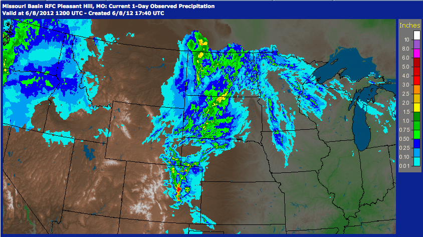
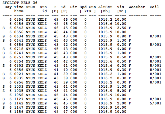
Parts of the north-central US (namely, western and central North Dakota and South Dakota, and far eastern Montana and Wyoming) received upwards of 0.5 to 1.0 inch of rainfall (Radar estimated precipitation | Regional temperature/precipitation data) in association with a slow-moving frontal boundary on 07 June 2012. With moist soil and strong radiational cooling during the following night (overnight lows included 43 F at Williston, North Dakota, 42 F at Hoover, South Dakota, and 38 F at Medicine Lake, Montana), areas of fog and low stratus clouds developed during the pre-dawn hours on 08 June 2012. AWIPS images of 1-km resolution GOES-13 0.63 µm visible channel data (above; click image to play animation) showed that these fog and low stratus cloud features quickly dissipated after sunrise with solar heating and increasing southeasterly winds.

A comparison of 4-km resolution GOES-13 and 375-meter resolution Suomi NPP VIIRS brightness temperature difference (BTD) “fog/stratus product” images just after 09 UTC or 4 AM local time (below) demonstrated the advantage of higher spatial resolution data for (1) depicting the formation of the more subtle valley fog features, and (2) more accurately defining the edges of low stratus cloud features.

GOES-13 vs Suomi NPP VIIRS "fog/stratus product" images

A comparison of the Suomi NPP VIIRS “fog/stratus product” with the corresponding 0.7 µm Day/Night Band (DNB) image (below) showed that with the moon in the waning gibbous phase (75% of full moon), the vertically-thicker low stratus cloud features in the western portion of the satellite scene were more brightly illuminated that the areas of thinner valley fog. It is also interesting to note the widespread bright DNB features associated with natural gas flares and illuminated man camps that are part of the extensive drilling operations across the Bakkan oil shale field (primarily in northwestern North Dakota; MSNBC news story).

Suomi NPP VIIRS "fog/stratus product" and Day/Night Band images

View only this post Read Less

GOES-12 10.7 µm IR image using Side 1 electronics (left) and Side 2 electronics (right)

At 1645 UTC on 6 June, an Electronics Side Swap occurred for GOES-12 to mitigate the effects of Cycle Slips that were occurring around 0800-1300 UTC each day (See this link for an explanation). No Cycle Slips occurred in the GOES-12 imager data on 7 June; as a result, the images are much cleaner. The image above shows an enhanced 10.7 µm image from June 4 2012 using the Side 1 electronics, which side was plagued by cycle slips, and from June 7 2012 using the Side 2 electronics, which show no cycle slips.

GOES-12 Imager (all channels) for 0945 UTC on June 4th and on June 7th (click image to play animation)

The Cycle Slips affected all bands. Click the image above to see the improvement across all bands between 0945 UTC on 4 June and 0945 UTC on 7 June. Note that there will be slight differences for a given input radiance in the computed brightness temperature for each band for the Side 2 Planck conversion coefficients versus the Side 1 Planck conversion coefficients. Those differences are, for Band 2, 0.0001K for both detectors; for Band 3, -0.0001 K for detector ‘a’, 0.0631 K for detector ‘b’; for Band 4, -0.0001 K for both detectors and for Band 6, 0.0119 K. These differences are much smaller than the instrument noise.

Real-time imagery of GOES-South America imager and sounder data are available here.

View only this post Read Less

POES AVHRR 12.0 µm IR image + SPC storm reports + METAR surface reports

Severe thunderstorms developed during the afternoon hours over eastern Colorado on 06 June 2012, which were responsible for a number of tornadoes in addition to widespread large hail and damaging winds (SPC storm reports). An AWIPS image of 1-km resolution POES AVHRR 12.0 µm IR channel data (above) showed a very pronounced “enhanced-V” storm top signature, with many of the severe weather reports located near the vertex of the enhanced-V.

A comparison of 1-km resolution POES AVHRR Cloud Top Temperature (CTT), Cloud Top Height (CTH), and Cloud Type products is shown below. The CTT cold/warm thermal couplet associated with the enhanced-V signature was -74 C/-55 C; the CTH values for the majority of the cirrus canopy were 13 km (12 km within the “warm spot” region of the enhanced-V); and the Cloud Type for the majority of the cirrus canopy was Overshooting (violet color enhancement), with the “Thick Ice” classification (yellow enhancement) within the warm region of the enhanced-V.

POES AVHRR Cloud Top Temperature, Cloud Top Height, and Cloud Type products

A comparison of the 1-km resolution POES 12.0 µm IR image with the corresponding 4-km resolution GOES-15 10.7 µm IR image (below) demonstrated the advantage of improved spatial resolution for detecting the more subtle aspects of the enhanced-V feature. Also note that the enhanced-V feature is displaced to the north and east on the GOES-15 image, due to the problem of parallax associated with the large viewing angle from the GOES-West satellite.

GOES-15 10.7 µm IR + POES AVHRR 12.0 µm IR images

The GOES-15 satellite was placed into Super Rapid Scan Operations (SRSO) mode, providing images as frequently as every 1 minute (see the VISIT Meteorological Interpretation Blog).

View only this post Read Less

GOES-13 11-3.9 µm legacy "fog/stratus product" (click image to play animation)

AWIPS images of the 4-km resolution GOES-13 11-3.9 µm brightness temperature difference (BTD) or “legacy fog/stratus product” (above; click image to play animation) began to display a signal of increasing coverage of fog and/or stratus across parts of the Allegheny Plateau region of New York and Pennsylvania during the pre-dawn hours of 06 June 2012. Strong nocturnal radiational cooling — Bradford, Pennsylvania (station identifier KBFD)  dropped to an overnight low temperature of 37 F — was helping to promote the formation of valley fog.

A more quantitative alternative to the legacy  BTD “fog/stratus product” is a new GOES Instrument Flight Rules (IFR) Probability product, developed as part of ASPB/CIMSS participation in the GOES-R Proving Ground. Note that the legacy fog/stratus product cannot make the distinction between fog and elevated stratus features (such as those found northwest of Lake Ontario, and also in west central Pennsylvania) — but the IFR Probability product does accurately make this discrimination. A trend of increasing areal coverage and magnitude of IFR Probability was noted (below; click image to play animation), especially along the New York/Pennsylvania border region where locations across southern New York such as Wellville (station identifier KELZ), Elmira (station identifier KELM), and Binghamton (station identifier KBGM) had surface visibilities drop to 1/4 mile and cloud ceilings drop to 100-200 feet above ground level.

GOES-13 IFR Probability product (click image to play animation)

A comparison of 4-km resolution GOES-13 and the corresponding 1-km resolution POES AVHRR “fog/stratus product” images at 07:40 UTC or 3:40 AM local time (below) demonstrated the importance of improved spatial resolution for the detection of small-scale features such as valley fog.

POES AVHRR vs GOES-13 legacy BTD "fog/stratus product" images

Similarly, a comparison of 4-km resolution GOES-13 and the corresponding 375-meter resolution (projected onto a 1-km resolution AWIPS grid) “fog/stratus product” images just after 08:00 UTC or 4:00 AM local time (below) showed much greater detail associated with the narrow fingers of valley fog.

Suomi NPP VIIRS vs GOES-13 legacy BTD "fog/stratus product" images

In addition, comparing the Suomi NPP VIIRS “fog/stratus product” with the VIIRS 0.7 µm Day/Night Band (DNB) image at that same time (below) showed that the DNB channel could detect a few of the narrow fingers of valley fog in far southwestern Pennsylvania and far northern Maryland that were obscured by high cirrus clouds (black features) on the “fog/stratus product” image. During periods of strong illumination from moonlight (as was the case on 06 June), the DNB can serve as a form of night-time visible channel imagery.

Suomi NPP VIIRS legacy BTD "fog/stratus product" vs VIIRS Day/Night Band image

After sunrise, McIDAS images of GOES-13 0.63 µm visible channel data (below; click image to play animation) showed the widespread valley fog features across parts of New York and Pennsylvania, which subsequently dissipated with daytime heating and boundary layer mixing.

GOES-13 0.63 µm visible channel images (click image to play animation)

View only this post Read Less