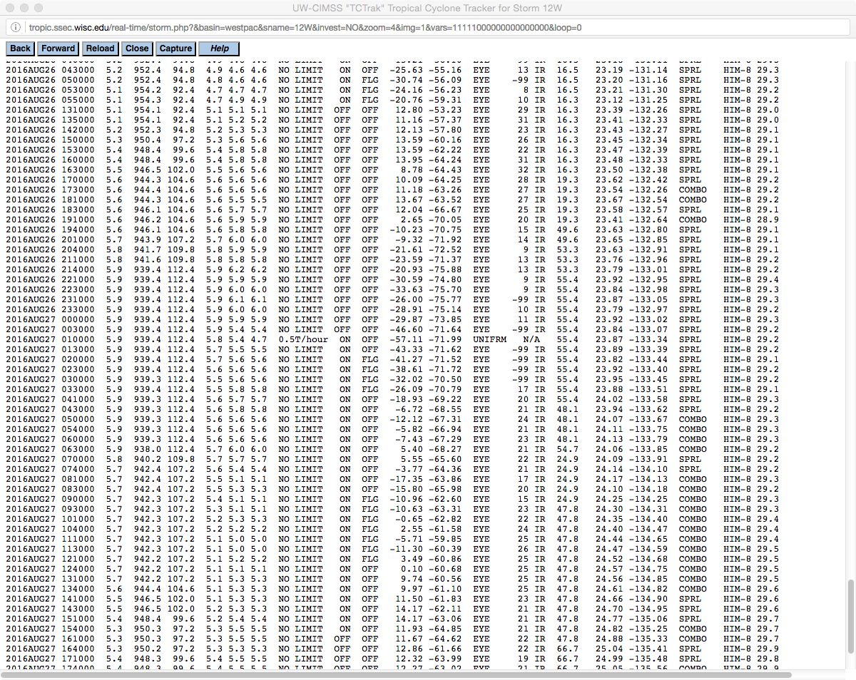
This website works best with a newer web browser such as Chrome, Firefox, Safari or Microsoft Edge. Internet Explorer is not supported by this website.

Major lake effect snow event downwind of Lake Erie and Lake Ontario

Cold arctic air (surface air temperatures in the upper teens to lower 20s F) flowing across the still-warm waters of Lake Erie and Lake Ontario (sea surface temperature values as warm as the middle to upper 40s F) were 2 ingredients that helped create... Read More

GOES-13 0.63 µm visible channel images (click to play animation)

GOES-13 0.63 µm visible channel images (click to play animation)

Cold arctic air (surface air temperatures in the upper teens to lower 20s F) flowing across the still-warm waters of Lake Erie and Lake Ontario (sea surface temperature values as warm as the middle to upper 40s F) were 2 ingredients that helped create a major lake effect snowfall event on 18 November 2014 (VIIRS visible image with surface analysis). Storm total snowfall amounts were as high as 65 inches in Erie County, New York (NWS Buffalo Public Information Statement). GOES-13 0.63 µm visible channel images (above; click image to play animation) showed the large and well defined single-band lake effect cloud features that developed over each of the lakes. The band over Lake Erie was nearly stationary for several hours, producing snowfall rates as high as 4 inches per hour at some locations in the Southtowns of Buffalo. The stationary behavior (and very sharp northern edge, due to a “locked thermal convergence zone“) of the Lake Erie snow band was quite evident on composite radar reflectivity (below; click image to play animation; images courtesy of the College of DuPage). The formation and growth of this band benefited from a long fetch of southwesterly winds oriented along the axis of Lake Erie.  Isolated negative cloud-to-ground lightning strikes were observed at 16:45 and 22:15 UTC, implying the presence of embedded pockets of thundersnow.

Composite radar reflectivity (click to play animation)

Composite radar reflectivity (click to play animation)

A comparison of Suomi NPP VIIRS 0.64 µm visible channel and 11.45 µm IR channel images at 18:17 UTC or 1:17 pm local time is shown below. The coldest cloud-top IR brightness temperature was -37º C (green color enhancement), which corresponded to a pressure of 437 hPa (or an altitude around 6 km) on the 12 UTC Buffalo NY rawinsonde report.

Suomi NPP VIIRS 0.64 µm visible channel and 11.45 µm IR channel images

Suomi NPP VIIRS 0.64 µm visible channel and 11.45 µm IR channel images

Comparisons of Terra and Aqua MODIS true-color Red/Green/Blue (RGB) images covering the Lake Erie/Lake Ontario region along with a high-resolution view centered on Buffalo NY are shown below.

Terra and Aqua MODIS true-color RGB images

Terra and Aqua MODIS true-color RGB images

Terra and Aqua MODIS true-color RGB images

Terra and Aqua MODIS true-color RGB images

A 15-meter resolution Landsat-8 0.59 µm panochromatic visible channel image from the SSEC RealEarth web map server (below) showed great detail to the Lake Ontario snow band as it was moving inland over the Watertown NY area at 15:45 UTC.

Landsat-8 0.59 µm panochromatic visible image

Landsat-8 0.59 µm panochromatic visible image

Looking back to the preceding nighttime hours, a toggle between Suomi NPP VIIRS 0.7 µm Day/Night Band, 3.74 µm shortwave IR, 11.45 µm IR, and 11.45-3.74 µm IR brightness temperature difference “Fog/stratus product” images at 06:54 UTC or 1:54 am local time (below) showed that the lake effect bands were already well-developed, with minimum 11.45 µm IR brightness temperatures of -30º C and colder (yellow color enhancement). Even with minimal lunar illumination — the Moon was in the Waning Crescent phase, at only 7% of full — the lake effect cloud bands features could still be seen on the Day/Night Band image.

Suomi NPP VIIRS 0.7 µm Day/Night Band, 3.74 µm shortwave IR, 11.45 µm IR, and

Suomi NPP VIIRS 0.7 µm Day/Night Band, 3.74 µm shortwave IR, 11.45 µm IR, and “Fog/stratus product” images

For a more in-depth discussion of this lake effect snow event, watch the VISIT Satellite Chat session.

View only this post Read Less

Eruption of the Pavlof Volcano in Alaska

According to the Alaska Volcano Observatory, an eruption of the Pavlof Volcano began around 01:50 UTC on 13 November 2014. A comparison of nighttime images of Suomi NPP VIIRS 0.7 µm Day/Night Band (DNB) and 3.74 µm shortwave IR data at 13:07 UTC... Read More

Suomi NPP VIIRS 0.7 µm Day/Night Band and 3.74 µm shortwave IR images

Suomi NPP VIIRS 0.7 µm Day/Night Band and 3.74 µm shortwave IR images

According to the Alaska Volcano Observatory, an eruption of the Pavlof Volcano began around 01:50 UTC on 13 November 2014. A comparison of nighttime images of Suomi NPP VIIRS 0.7 µm Day/Night Band (DNB) and 3.74 µm shortwave IR data at 13:07 UTC or 4:07 am local time on 14 November (above) showed the bright glow of the eruption on the DNB image, with the hottest pixel being 52º C (red color enhancement) on the shortwave IR image.

With the subsequent arrival of daylight, a break in the clouds allowed the faint volcanic plume to be observed on GOES-15 0.63 µm visible channel images (below; click image to play animation), drifting northwestward over the Bering Sea.

GOES-15 0.63 µm visible channel images (click to play animation)

GOES-15 0.63 µm visible channel images (click to play animation)

At 22:02 UTC on 14 November, the radiometrically-retrieved maximum volcanic ash mass loading value was 1.8 tons per km2, the maximum ash height was 16.8 km, and the maximum ash mass effective radius was 7.81 µm (below).

MODIS volcanic ash mass loading, ash height, and ash mass effective radius products

MODIS volcanic ash mass loading, ash height, and ash mass effective radius products

About an hour later, the volcanic ash plume could be seen on a 23:03 UTC Suomi NPP VIIRS Day/Night Band image, with a maximum 3.74 µm shortwave IR brightness temperature of 46º C at the summit of the volcano (below).

Suomi NPP VIIRS 0.7 µm Day/Night Band and 3.74 µm shortwave IR images

Suomi NPP VIIRS 0.7 µm Day/Night Band and 3.74 µm shortwave IR images

The brown hue of the volcanic ash plume was very evident on Suomi NPP VIIRS true-color Red/Green/Blue (RGB) images from the SSEC RealEarth web map server (below).

Suomi NPP VIIRS true-color RGB images

Suomi NPP VIIRS true-color RGB images

The intensity of the Pavlof eruption increased on 15 November, and a well-defined volcanic ash plume could be seen on GOES-15 0.63 µm visible channel images (below; click image to play animation). Pilot reports estimated that the top of the plume was as high as 38,000 feet.

GOES-15 0.63 µm visible channel images (click to play animation)

GOES-15 0.63 µm visible channel images (click to play animation)

On a comparison of Suomi NPP VIIRS 0.64 µm visible channel and 11.45 µm IR channel images at 22:45 UTC (below), the coldest cloud-top IR brightness temperature value was -55º C.

Suomi NPP VIIRS 0.64 µm visible channel and 11.45 µm IR channel images

Suomi NPP VIIRS 0.64 µm visible channel and 11.45 µm IR channel images

At 22:29 UTC, the CLAVR-x POES AVHRR Cloud Top Temperature product indicated a minimum value of -54º C, with a maximum Cloud Top Height value of 9 km; the -54º C cloud top temperature corresponded to an altitude of around 29,000 feet or 8.7 km on the 16 November/00 UTC Cold Bay AK rawinsonde profile.

POES AVHRR Cloud Top Temperature and Cloud Top Height products

POES AVHRR Cloud Top Temperature and Cloud Top Height products

A Suomi NPP VIIRS true-color RGB image at 23:04 UTC (below) suggested that the volcanic plume consisted of a dense layer of tan-colored ash, with a layer of mostly ice cloud at the top of the plume.

Suomi NPP VIIRS true-color RGB image

Suomi NPP VIIRS true-color RGB image

View only this post Read Less

“River-effect” snow in South Dakota

GOES-13 0.63 µm visible channel images (above; click image to play animation) revealed the presence of numerous cloud streamers originating over the Lake Oahe and Lake Sharpe reservoirs along the Missouri River in South Dakota on 13 November 2014. At times these cloud... Read More

GOES-13 0.63 µm visible channel images (click to play animation)

GOES-13 0.63 µm visible channel images (click to play animation)

GOES-13 0.63 µm visible channel images (above; click image to play animation) revealed the presence of numerous cloud streamers originating over the Lake Oahe and Lake Sharpe reservoirs along the Missouri River in South Dakota on 13 November 2014. At times these cloud bands were producing snow that was reducing surface visibility to 4 miles at Pierre (KPIR) and 5 miles at Chamberlain (K9V9).

Aqua MODIS 0.65 µm visible channel image, False-color RGB image, and Sea Surface Temperature product at 19:48 UTC

Aqua MODIS 0.65 µm visible channel image, False-color RGB image, and Sea Surface Temperature product at 19:48 UTC

Comparisons of visible channel and false-color Red/Green/Blue (RGB) images from Aqua MODIS (above) and Suomi NPP VIIRS (below) demonstrated the value of RGB products to more easily identify such supercooled water droplet cloud features (which appear as varying shades of white) in areas that have underlying snow cover (which appears as varying shades of red). In addition, the MODIS Sea Surface Temperature (SST) product (above) showed that SST values were in the 40-50º F range (cyan color enhancement) in those Missouri River reservoirs, making them significantly warmer than the cold arctic air mass that had overspread the region.

Suomi NPP VIIRS 0.64 µm visible channel image and False-color RGB image at 19:51 UTC

Suomi NPP VIIRS 0.64 µm visible channel image and False-color RGB image at 19:51 UTC

View only this post Read Less

Displaying NUCAPS data from CLASS

NUCAPS data have been flowing into AWIPS 2 for months; in the recent past, these data started flowing into the NOAA CLASS data archive as well (click here for a tutorial on accessing the data). How can the NOAA CLASS output be displayed? This post will compare McIDAS-V plots to the data displayed using AWIPS-1, below.Suomi NPP overflew... Read More

NUCAPS data have been flowing into AWIPS 2 for months; in the recent past, these data started flowing into the NOAA CLASS data archive as well (click here for a tutorial on accessing the data). How can the NOAA CLASS output be displayed? This post will compare McIDAS-V plots to the data displayed using AWIPS-1, below.

GOES Sounder Total Column Ozone DPI Values Plotted with NAM 500-mb heights and NAM Pressure on the 1.5 PVU surface (click to enlarge)

GOES Sounder Total Column Ozone DPI Values Plotted with NAM 500-mb heights and NAM Pressure on the 1.5 PVU surface (click to enlarge)

Suomi NPP overflew the central United States at about 0850 UTC on 12 November, and ozone concentrations from the NUCAPS soundings at three different levels (~500, 300 and ~200 mb) are shown below. Note that the color scaling is not quite the same in the three plots as the range for each pressure level is different. Maxima in Ozone at all levels occur in the same region — the Dakotas — as indicated by the GOES Sounder Total Column Ozone DPI, above. NUCAPS soundings also show data in cloudy regions because microwave data from ATMS is used in the NUCAPS processing. Note that values at the edge of the color shading have been extrapolated outwards; values in western Nevada and Indiana, for example, are not from direct NUCAPS observations. This plot of 500-mb temperatures (that includes the actual values) shows the horizontal extent of data and the amount of interpolation at the edge.

Contours of Ozone Mixing Ratio (parts per billion) from NUCAPS Soundings at ~0848 UTC on 12 November 2014 (click to enlarge)

Contours of Ozone Mixing Ratio (parts per billion) from NUCAPS Soundings at ~0848 UTC on 12 November 2014 (click to enlarge)

View only this post Read Less