The Pioneer Fire in central Idaho produced another pyroCumulonimbus (pyroCb) cloud on 21 August 2016 (the first was on 19 August). GOES-14 was in SRSO-R mode, and sampled the fire with 1-minute imagery (above; also available as a large 73 Mbyte animated GIF) — a large smoke plume was evident on 0.63 µm Visible images as... Read More

GOES-14 0.63 µm Visible (top), 3.9 µm Shortwave Infrared (middle) and 10.7 µm Infrared Window (bottom) images, with surface reports plotted in yellow [click to play MP4 animation]
The
Pioneer Fire in central Idaho produced another pyroCumulonimbus (pyroCb) cloud on
21 August 2016 (the first was on
19 August). GOES-14 was in
SRSO-R mode, and sampled the fire with 1-minute imagery
(above; also available as a large 73 Mbyte animated GIF) — a large smoke plume was evident on 0.63 µm Visible images as it moved eastward; large fire hot spots
(red pixels) were seen on 3.9 µm Shortwave Infrared images; on 10.7 µm Infrared Window images, the cloud-top IR brightness temperature cooled to -35º C
(darker green enhancement) between 2249-2307 UTC as it moved over Stanley Ranger Station (KSNY), not quite reaching the -40º C threshold to be classified as a pyroCb.
However, a 1-km resolution NOAA-19 AVHRR 10.8 µm Infrared Window image (below; courtesy of René Servranckx) revealed a minimum cloud-top IR brightness temperature of -48.3º C (dark green color enhancement).
![NOAA-19 AVHRR 0.64 µm visible (top left), 3.7 µm shortwave IR (top right), 10.8 µm IR window (bottom left) and false-color RGB composite image (bottom right) [click to enlarge]](http://pyrocb.ssec.wisc.edu/wp-content/uploads/2016/08/20160821_2201utc_Ch1_ch3_ch4_ch321.jpg)
NOAA-19 AVHRR 0.64 µm visible (top left), 3.7 µm shortwave IR (top right), 10.8 µm IR window (bottom left) and false-color RGB composite image (bottom right) [click to enlarge]
A larger-scale comparison of the NOAA-19 AVHRR visible, shortwave infrared and infrared window images is shown below.
![NOAA-19 Visible (0.63 µm), Shortwave Infrared (3.7 µm) and Infrared Window (10.8 µm) images [click to enlarge]](https://cimss.ssec.wisc.edu/satellite-blog/wp-content/uploads/sites/5/2016/08/160821_2158utc_noaa19_vis_swir_ir_ID_pyrocb_anim.gif)
NOAA-19 Visible (0.63 µm), Shortwave Infrared (3.7 µm) and Infrared Window (10.8 µm) images [click to enlarge]
===== 23 August Update =====
![Suomi NPP VIIRS Shortwave Infrared (3.74 µm), Day/Night Band (0.7 µm) and 11.45-3.74 µm brightness temperature difference images [click to enlarge]](https://cimss.ssec.wisc.edu/satellite-blog/wp-content/uploads/sites/5/2016/08/160823_1032utc_suomi_npp_viirs_swir_dnb_fog_Pioneer_Fire_ID_anim.gif)
Suomi NPP VIIRS Shortwave Infrared (3.74 µm), Day/Night Band (0.7 µm) and 11.45-3.74 µm brightness temperature difference images [click to enlarge]
The Pioneer Fire continued to be very active on
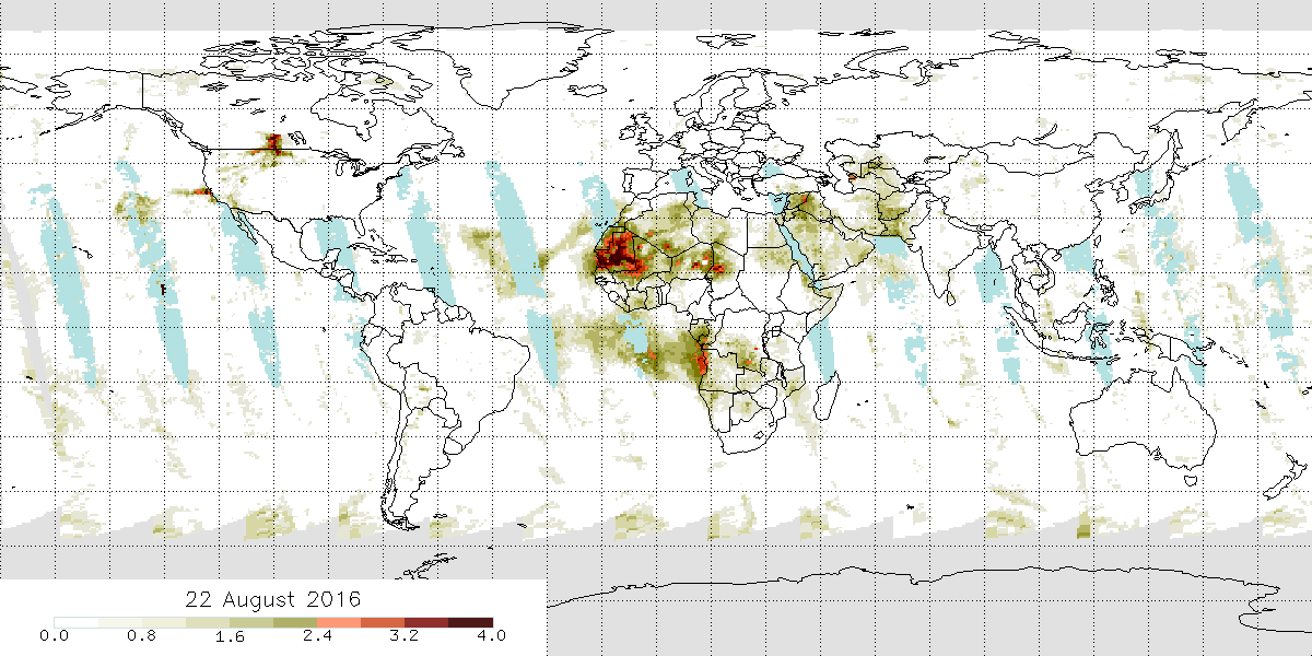
22 August (exceeding 100,000 acres in total burn coverage since its start on 18 July), sending a large amount of smoke northeastward (
OMPS Aerosol Index). During the following overnight hours, cold air drainage and the development of a boundary layer temperature inversion acted to trap a good deal of smoke in the Payette River valley to the west/southwest of Stanley KSNT. The active fire hot spots
(black to yellow to red pixels) were evident on nighttime (1032 UTC or 4:32 AM local time) images
(above) of Suomi NPP VIIRS Shortwave Infrared (3.74 µm) data, while illumination from the Moon (in the Waning Gibbous phase, at 69% of Full) showed the ribbon of smoke trapped in the valley (note that this signal was not due to fog, since it did not show up in the VIIRS 11.45-3.74 µm brightness temperature difference or “fog/stratus product”).
During the subsequent daytime hours of 23 August, 1-minute GOES-14 Visible (0.63 µm) images (below; also available as a large 114 Mbyte animated GIF) showed the gradual ventilation of smoke from the Payette River valley as the temperature inversion eroded and mixing via winds increased.
![GOES-14 Visible (0.63 um) images, with plots of hourly surface reports [click to play MP4 animation]](https://cimss.ssec.wisc.edu/satellite-blog/wp-content/uploads/sites/5/2016/08/960x1280_GOES14_B1_GOES14_VIS_ID_SMOKE_23AUG2016_2016236_150200_0001PANEL.GIF)
GOES-14 Visible (0.63 um) images, with plots of hourly surface reports [click to play MP4 animation]
View only this post
Read Less
![GOES-14 0.63 µm Visible (top), 3.9 µm Shortwave Infrared (middle) and 10.7 µm Infrared Window (bottom) images [click to play MP4 animation]](http://pyrocb.ssec.wisc.edu/wp-content/uploads/2016/08/GOES14_VIS_SWIR_IR_3PANEL_CA_FIRE_22AUG2016_320x1280_B124_00152_2016235_222500_222500_222500_0003PANELS.GIF)
![Vandenberg Air Force Base rawinsonde report [click to enlarge]](http://pyrocb.ssec.wisc.edu/wp-content/uploads/2016/08/160823_00Z_72393_KVBG_RAOB.GIF)
![Suomi NPP VIIRS true-color and false-color images [click to enlarge]](http://pyrocb.ssec.wisc.edu/wp-content/uploads/2016/08/160822_2036utc_viirs_truecolor_falsecolor_Rey_Fire_CA_anim.gif)
![GOES-14 Visible (0.63 µm) images, with hourly surface weather symbols plotted in yellow [click to play MP4 animation]](https://cimss.ssec.wisc.edu/satellite-blog/wp-content/uploads/sites/5/2016/08/960x1280_GOES14_B1_GOES14_VIS_PACNW_17AUG2016_2016230_172600_0001PANEL.GIF)
![GOES-14 Visible (0.63 µm) images, with hourly plots of surface reports in yellow [click to play MP4 animation]](https://cimss.ssec.wisc.edu/satellite-blog/wp-content/uploads/sites/5/2016/08/960x1280_GOES14_B1_GOES14_VIS_SFO_17AUG2016_2016230_160400_0001PANEL.GIF)
![GOES-14 0.63 µm Visible (left) and 3.9 µm Shortwave Infrared (right) images, with hourly plots of surface reports in cyan/yellow [click to play MP4 animation]](https://cimss.ssec.wisc.edu/satellite-blog/wp-content/uploads/sites/5/2016/08/960x640_GOES14_B12_GOES14_VIS_SWIR_CA_FIRE_16AUG2016_2016230_154500_0002PANELS.GIF)
![GOES-14 Visible (0.63 µm) images, with county outlines and 4-character airport identifiers [click to play MP4 animation]](https://cimss.ssec.wisc.edu/satellite-blog/wp-content/uploads/sites/5/2016/08/960x1280_GOES14_B1_GOES14_VIS_BLUE_CUT_FIRE_CA_17AUG2016_2016230_213200_0001PANEL.GIF)
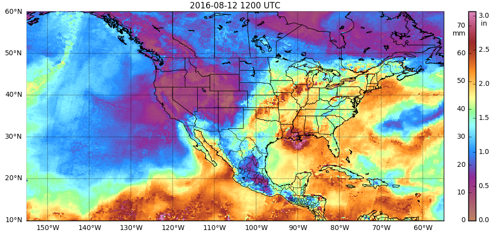
![Morphed MIRS observations of total precipitable water (TPW), 1500 UTC 11 August - 2100 UTC 12 August [click to play animation]](https://cimss.ssec.wisc.edu/satellite-blog/wp-content/uploads/sites/5/2016/08/MIMICTPw_0811_15_0812_21anim.gif)
![GOES-14 Visible (0.62 µm) images, with METAR observations of 6-hour precipitation, 1200 and 1800 UTC on 12 August 2016 [click to enlarge]](https://cimss.ssec.wisc.edu/satellite-blog/wp-content/uploads/sites/5/2016/08/PRECIPTOTAL_12_18_12August2016toggle.gif)
![GOES-14 Infrared Window (10.7 µm) Imagery, 1625-1830 UTC on 12 August 2016 [click to play animation]](https://cimss.ssec.wisc.edu/satellite-blog/wp-content/uploads/sites/5/2016/08/GOES14_12AUG_IR4_12Aug_1625_1830anim.gif)
![GOES-14 Infrared Window (10.7 µm) images, with surface weather symbols plotted in yellow [click to play MP4 animation]](https://cimss.ssec.wisc.edu/satellite-blog/wp-content/uploads/sites/5/2016/08/960x1280_AGOES14_B4_GOES14_IR_LA_12AUG2016_2016225_235800_0001PANEL.GIF)
![GOES-14 Infrared Window (10.7 µm) images, with hourly surface weather symbols plotted in yellow [click to play MP4 animation]](https://cimss.ssec.wisc.edu/satellite-blog/wp-content/uploads/sites/5/2016/08/960x1280_AGOES14_B4_GOES14_IR_LA_11-13AUG2016_2016226_111500_0001PANEL.GIF)
