GOES-16 and GOES-17 satellite imagery can be remapped and combined to create stereoscopic imagery. To achieve the 3-dimensional effect, cross your eyes until three scenes are visible, and focus on the middle image. You can also achieve this by placing a finger halfway between your eyes and the screen, and... Read More

GOES-16 (left) and GOES-17 (right) visible (0.64 µm) imagery on 24 October 2019, 1500-2350 UTC (Click to animate)
GOES-16 and GOES-17 satellite imagery can be remapped and combined to create stereoscopic imagery. To achieve the 3-dimensional effect, cross your eyes until three scenes are visible, and focus on the middle image. You can also achieve this by placing a finger halfway between your eyes and the screen, and focusing on your finger, then focusing on the image behind. (Here’s a website that might help). The imagery above, from 24 October 2019, shows high clouds rotating anti-cyclonically above the smoke produced from the Kincade Fire (previous blog posts on this fire are here and here). The smoke plume extended far out into the Pacific Ocean. A Full-resolution image animation is shown below.

GOES-16 (left) and GOES-17 (right) visible (0.64 µm) imagery on 24 October 2019, 1500-2350 UTC (Click to animate)
Animations for 25 October, 26 October, 27 October, 28 October and 29 October are shown below, in order.

GOES-16 (left) and GOES-17 (right) visible (0.64 µm) imagery from 1500 UTC on 25 October 2019 to 0050 UTC on 26 October 2019 (Click to animate)
On the 25th and 26th of October, prevailing winds moved smoke into the Bay Area. On both days, the fire appeared less vigorous in the visible imagery than on the 24th, at top, or on the 27th; at least, it appeared to be producing less smoke.
GOES-16 (left) and GOES-17 (right) visible (0.64 µm) imagery from 1500 UTC on 26 October 2019 to 0050 UTC on 27 October 2019 (Click to animate)
On the 27th, below, the fire resembled the scene on 24 October, with a large smoke plume extending far southwest into the Pacific Ocean.
GOES-16 (left) and GOES-17 (right) visible (0.64 µm) imagery from 1500 UTC to 2350 UTC on 27 October 2019 (Click to animate)
On the 28th, below, smoke generation has decreased, and the smoke pall appears over the Bay Area again. A full-resolution version is available here.
GOES-16 (left) and GOES-17 (right) visible (0.64 µm) imagery from 1500 UTC to 2350 UTC on 28 October 2019 (Click to animate)
The scene on the 29th, below (Full resolution available here) is shown below. The smoke plume is extensive.
GOES-16 (left) and GOES-17 (right) visible (0.64 µm) imagery from 1500 UTC to on 29 October 2019 to 0050 UTC on 30 October 2019 (Click to animate)
How did the smoke plume change from day to day? The animation below shows data at 2350 UTC on 24-29 October.
GOES-16 (left) and GOES-17 (right) visible (0.64 µm) imagery at 2350 UTC from 24 to 29 October 2019 (Click to enlarge)
View only this post
Read Less
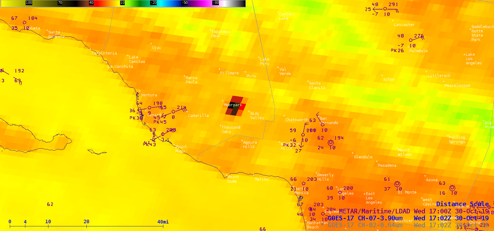
![GOES-17 Shortwave Infrared (3.9 µm) and “Red” Visible (0.64 µm) images [click to play animation | MP4]](https://cimss.ssec.wisc.edu/satellite-blog/wp-content/uploads/sites/5/2019/10/191030_goes17_visible_shortwaveInfrared_SoCal_fires_anim.gif)
![3.74 µm Shortwave Infrared images from Suomi NPP and NOAA-20 compared with the corresponding GOES-17 3.9 µm images [click to enlarge]](https://cimss.ssec.wisc.edu/satellite-blog/wp-content/uploads/sites/5/2019/10/191030_viirs_goes17_shotwaveInfrared_Easy_Fire_CA_anim.gif)


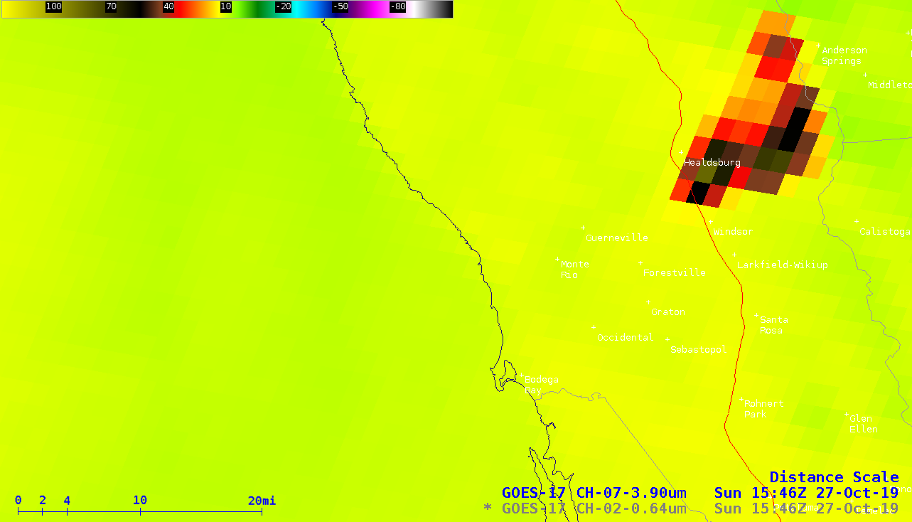
![GOES-17 Shortwave Infrared (3.9 µm) and “Red” Visible (0.64 µm) images [click to play animation | MP4]](https://cimss.ssec.wisc.edu/satellite-blog/wp-content/uploads/sites/5/2019/10/191027_goes17_shortwaveInfrared_visible_Kincade_Fire_CA_anim.gif)
![GOES-17 True Color RGB images [click to play animation | MP4]](https://cimss.ssec.wisc.edu/satellite-blog/wp-content/uploads/sites/5/2019/10/191027_goes17_trueColorRGB_Kincade_Fire_CA_anim.gif)
![VIIRS Shortwave Infrared (3.74 µm) images from Suomi NPP and NOAA-20 [click to enlarge]](https://cimss.ssec.wisc.edu/satellite-blog/wp-content/uploads/sites/5/2019/10/191026_191027_viirs_shortwaveInfrared_Kincade_Fire_CA_anim.gif)
