GOES-17 (GOES-West) Upper-level Water Vapor (6.2 µm) and Air Mass Red-Green-Blue (RGB) images (above) displayed a series of shear vortices migrating southward over the East Pacific Ocean (off the cost of the Pacific Northwest) on 24 November 2020. The ribbon of brighter orange to red hues on the RGB images highlight regions of dry, ozone-rich air where the tropopause... Read More
![GOES-17 Upper-level Water Vapor (6.2 µm) and Air Mass RGB images [click to play animation | <strong>MP4</strong>]](https://cimss.ssec.wisc.edu/satellite-blog/images/2020/11/epac_wv-20201124_180117.png)
GOES-17 Upper-level Water Vapor (6.2 µm) and Air Mass RGB images [click to play animation | MP4]
GOES-17
(GOES-West) Upper-level Water Vapor (
6.2 µm) and
Air Mass Red-Green-Blue (RGB) images
(above) displayed a series of shear vortices migrating southward over the East Pacific Ocean (off the cost of the Pacific Northwest) on
24 November 2020. The ribbon of brighter orange to red hues on the RGB images highlight regions of dry, ozone-rich air where the tropopause was at a significantly lower altitude compared to adjacent areas.
GOES-17 Water Vapor images with isotachs of NAM40 model maximum wind speed (below) showed that these vortices were forming within a very tight gradient in wind velocity (which existed just to the left of a southward-moving polar jet streak) — so speed shear was a mechanism playing a role.
![GOES-17 Upper-level Water Vapor (6.2 µm) images, with isotachs of NAM40 model maximum wind speed [click to enlarge]](https://cimss.ssec.wisc.edu/satellite-blog/images/2020/11/201124_goes17_waterVapor_nam40maxWindSpeed_East_Pacific_shear_vortices_anim.gif)
GOES-17 Upper-level Water Vapor (6.2 µm) images, with isotachs of NAM40 model maximum wind speed [click to enlarge]
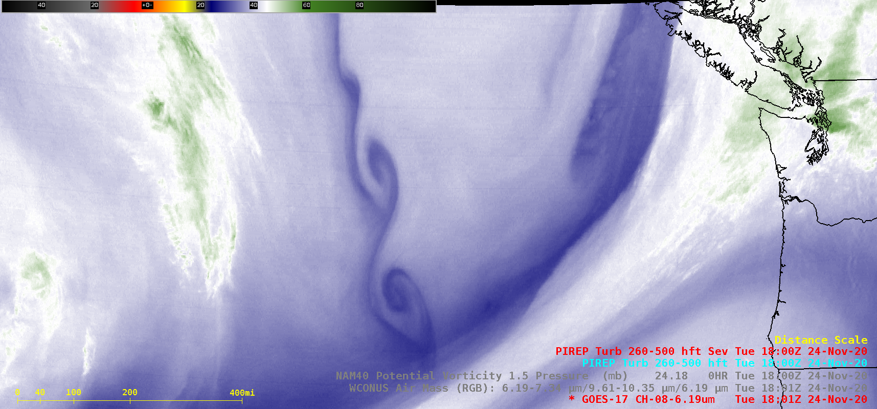
GOES-17 Air Mass RGB images with and without contours of NAM40 model PV1.5 pressure
(below) indicated that the dynamic tropopause descended to the 500-600 hPa level in the vicinity of the most well defined shear vortices. Occasionally aircraft encounter turbulence near these types of vortices — but in this case, there were no pilot reports of turbulence in those areas.
![GOES-17 Air Mass RGB images, with and without contours of NAM40 model PV1.5 pressure [click to play animation | MP4]](https://cimss.ssec.wisc.edu/satellite-blog/images/2020/11/epac_rgb-20201124_180117.png)
GOES-17 Air Mass RGB images, with and without contours of NAM40 model PV1.5 pressure [click to play animation | MP4]
View only this post
Read Less
![US Space Force EWS-G1 Infrared (10.7 µm) images [click to play animation | MP4]'](https://cimss.ssec.wisc.edu/satellite-blog/images/2020/11/201125_ewsg1_infrared_Cyclone_Nivar_landfall_anim.gif)
![Meteosat-8 Infrared Window (10.8 µm) images, with contours of deep-layer wind shear [click to enlarge]](https://cimss.ssec.wisc.edu/satellite-blog/images/2020/11/201125_meteosat8_infrared_shear_Cyclone_Nidar_anim.gif)
![GOES-17 Upper-level Water Vapor (6.2 µm) and Air Mass RGB images [click to play animation | <strong>MP4</strong>]](https://cimss.ssec.wisc.edu/satellite-blog/images/2020/11/201124_goes17_waterVapor_airMassRGB_East_Pacific_shear_vortices_anim.gif)
![GOES-17 Air Mass RGB images, with and without contours of NAM40 model PV1.5 pressure [click to play animation | MP4]](https://cimss.ssec.wisc.edu/satellite-blog/images/2020/11/201124_goes17_airMassRGB_pv1.5pressure_East_Pacific_shear_vortices_anim.gif)
![EUMETSAT Meteosat-11 High Resolution Visible (0.8 µm) images [click to play animation | MP4]](https://cimss.ssec.wisc.edu/satellite-blog/images/2020/11/201122_meteosat11_visible_Medicane_anim.gif)
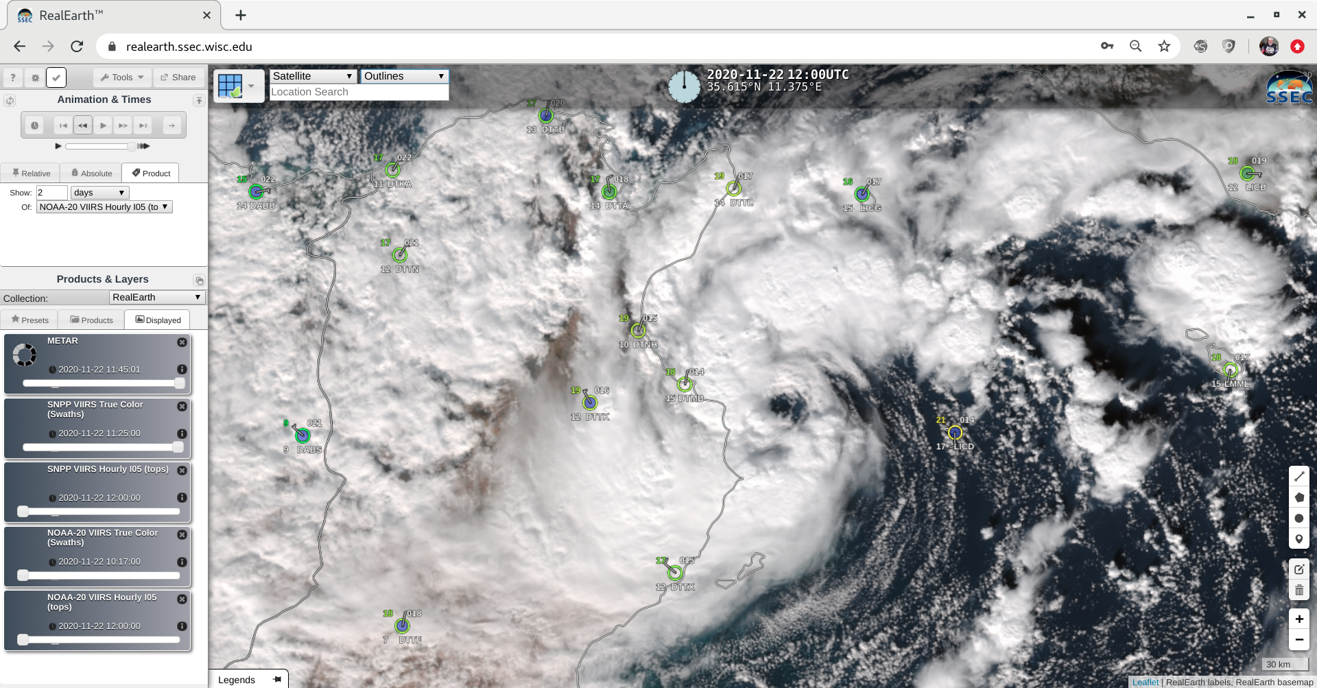
![Suomi NPP VIIRS True Color RGB image valid at 1152 UTC [click to enlarge]](https://cimss.ssec.wisc.edu/satellite-blog/images/2020/11/201122_1152utc_suomiNPP_viirs_trueColorRGB_medicane_anim.gif)
![Plot of surface observations for Monastir's Habib Bourguiba International Airport [click to enlarge]](https://cimss.ssec.wisc.edu/satellite-blog/images/2020/11/201122_DTMB_SFCMG.GIF)
![EWS-G1 Visible (0.63 µm) images [click to play animation | MP4]](https://cimss.ssec.wisc.edu/satellite-blog/images/2020/11/201122_ewsg1_visible_Cyclone_Gati_landfall_anim.gif)
![EWS-G1 Infrared Window (10.7 µm) images [click to play animation | MP4]](https://cimss.ssec.wisc.edu/satellite-blog/images/2020/11/201122_ewsg1_infrared_Cyclone_Gati_landfall_anim.gif)
