NOAA/CIMSS ProbSevere display, 1545 – 1700 UTC on 27 January 2021 (Click to animate)
A tornado struck the Tallahassee, FL, airport at 1643 UTC on 27 January 2021 (SPC Storm Report). The animation above shows ProbSevere (version 2) fields (from this site) in the hour leading up to tornadogenesis. The animation demonstrates how ProbTor values can be used to identify for closer scrutiny a particular radar object: the radar object that ultimately caused a tornado showed greater ProbTor values (than surrounding identified radar objects) in the hour leading up to tornadogenesis. In addition, ProbTor values ramped up quickly just prior to tornadogenesis as low-level azimuthal shear jumped.
One time series below compares ProbWind, ProbHail and ProbTor for the radar object (#15080) that produced the tornado; for this event, ProbWind and ProbTor values were comparable until a ramp-up in ProbTor values before the tornado occurred. The second time series shows the various components of ProbTor for radar object 15080 (both time series courtesy John Cintineo, SSEC/CIMSS). Note in particular that this storm was not a lightning-producer. Much of ProbTor’s variability was determined by changes in low-level azimuthal shear.
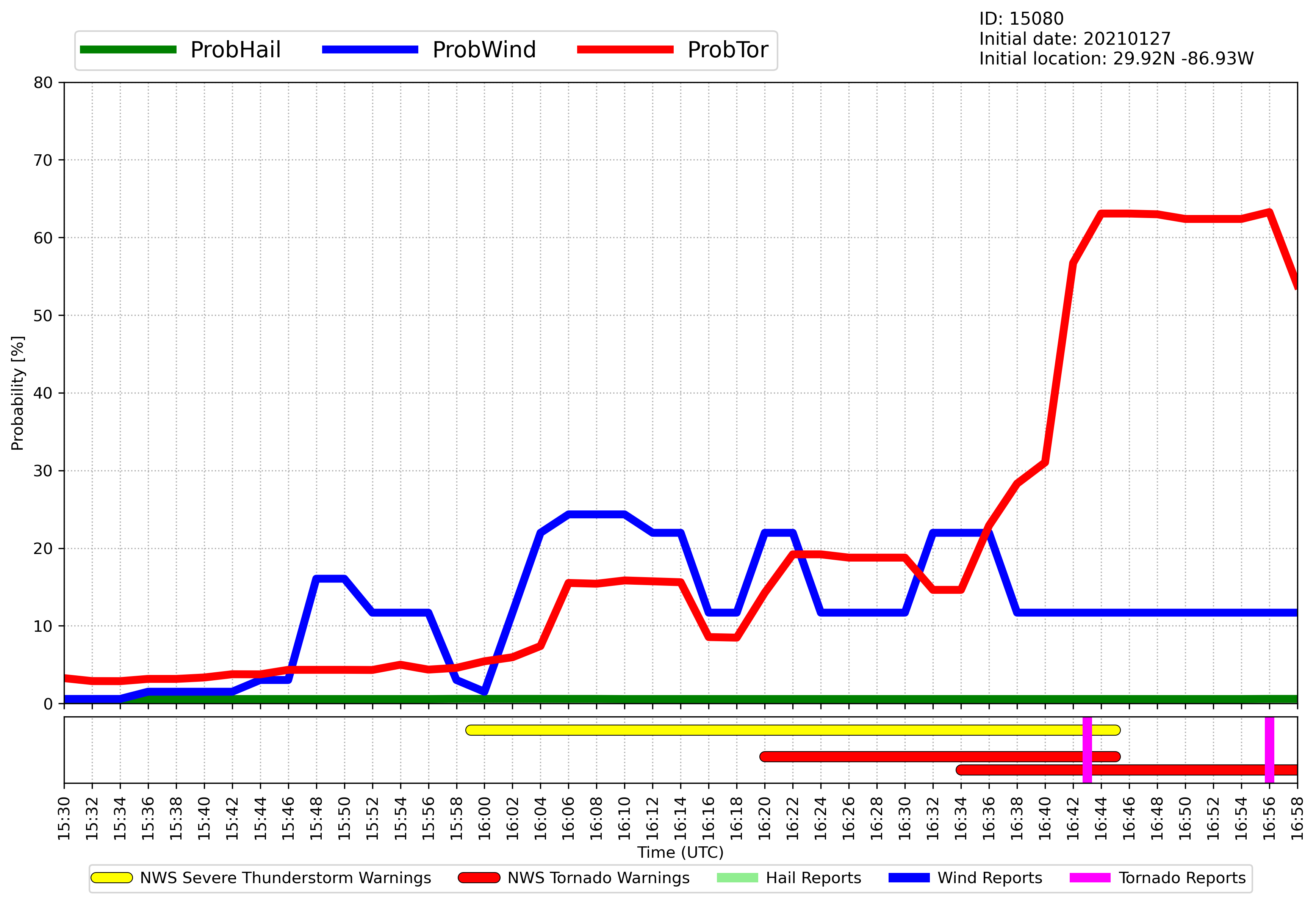
NOAA/CIMSS ProbSevere values (ProbWind, ProbHail, ProbTor) for radar object #15080, 1530 – 1658 UTC on 27 January 2021 (Click to enlarge)
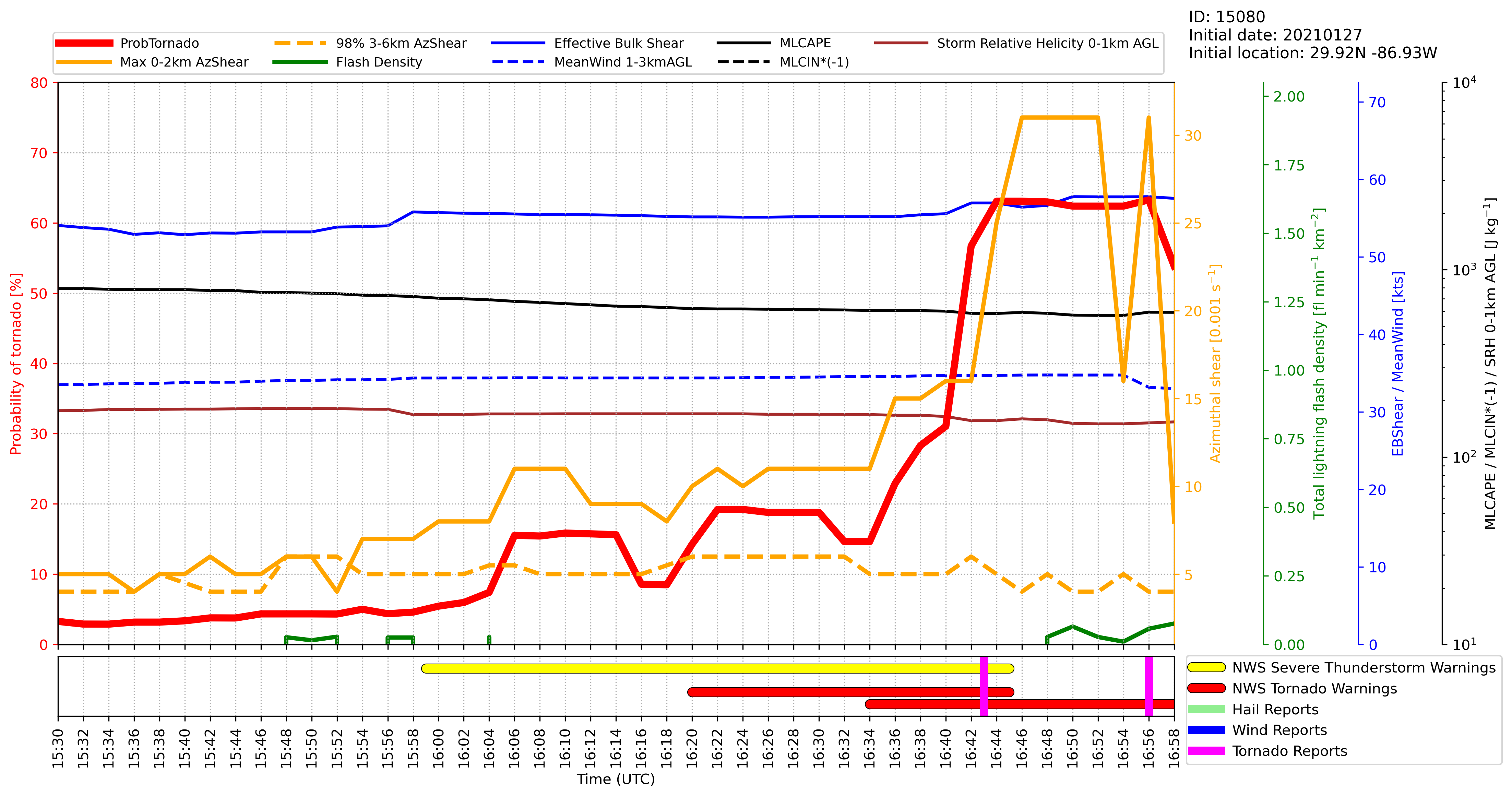
NOAA/CIMSS ProbTor and component values for Radar object #15080, 1530 – 1658 UTC on 27 January 2021, associated with the Tallahassee FL tornado (Click to enlarge)
Lead time with ProbTor in this example was not exceptional. However, its elevated values in the hour leading up to the tornado could have provided better situational awareness, and perhaps enhanced confidence in warning issuance for this well-warned event.
_________________________________________________________________________________________________________

GOES-16 “Red” Visible (0.64 µm, left) and “Clean” Infrared Window (10.35 µm, right) images, with plots of SPC Storm Reports [click to play animation | MP4]
There was an overpass of the Terra satellite about 19 minutes before the start of the tornado event, at 1618 UTC — 1-km resolution MODIS Visible (0.64 µm) and Infrared Window (11.0 µm) images are shown below.
![Terra MODIS Visible (0.64 µm) and Infrared Window (11.0 µm) images [click to enlarge]](https://cimss.ssec.wisc.edu/satellite-blog/images/2021/01/210127_1618uc_terra_modis_visible_infrared_TLH_anim.gif)
Terra MODIS Visible (0.64 µm) and Infrared Window (11.0 µm) images [click to enlarge]
View only this post Read Less

![GOES-16 "Clean" Infrared Window (10.35 um) images [click to play animation | MP4]](https://cimss.ssec.wisc.edu/satellite-blog/images/2021/01/210125_goes16_infrared_AL_anim.gif)
![Plot of 00 UTC rawinsonde data from Birmingham, Alabama [click to enlarge]](https://cimss.ssec.wisc.edu/satellite-blog/images/2021/01/210126_00utc_kbmx_raob.png)
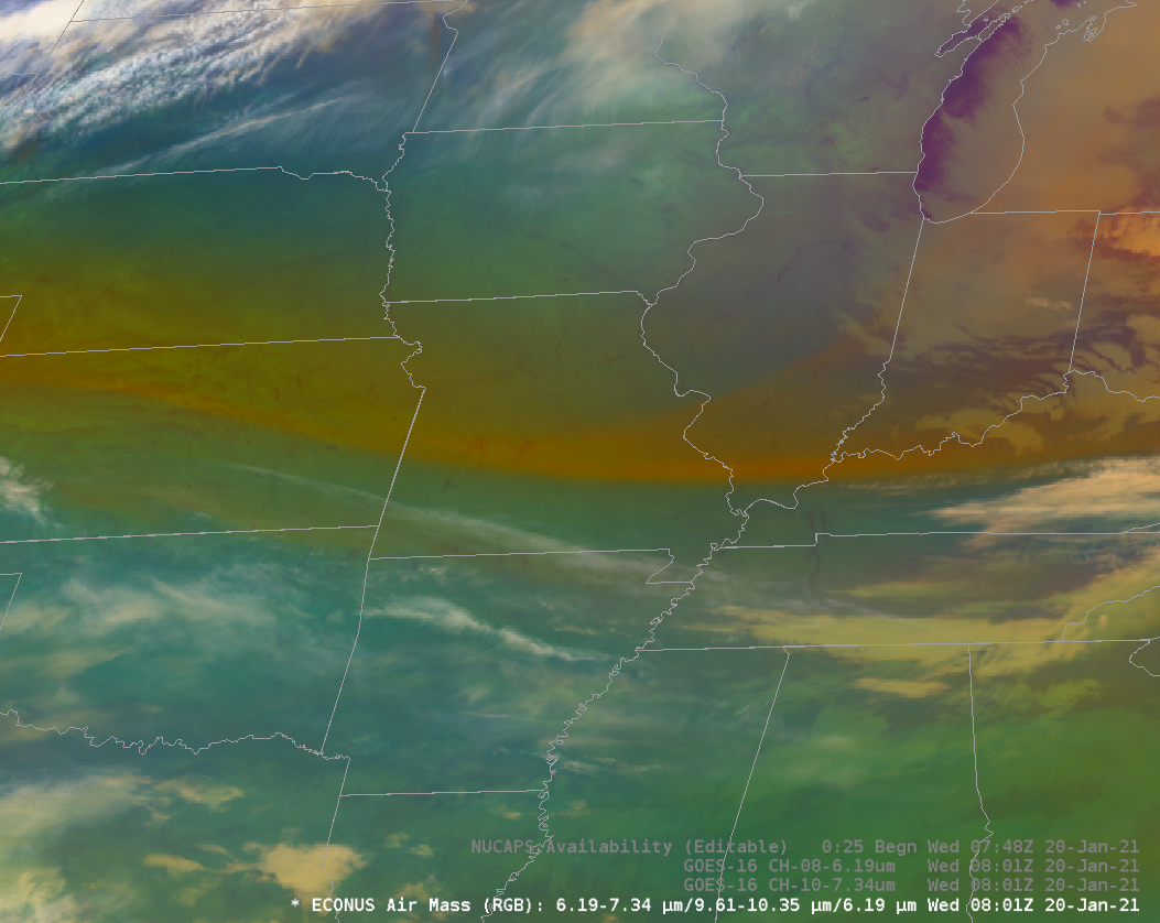
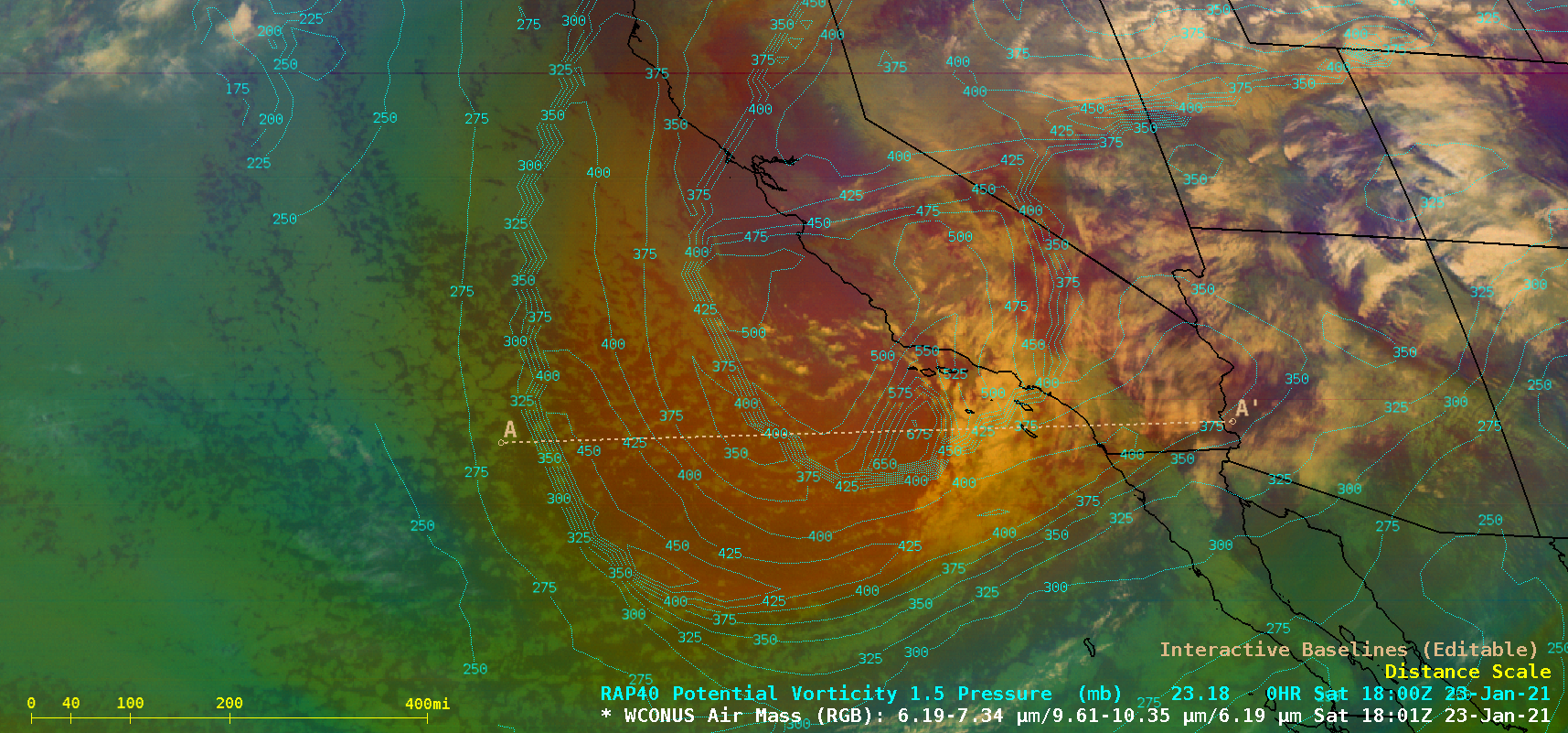
![GOES-17 Air Mass RGB images, with contours of PV1.5 pressure [click to play animation | MP4]](https://cimss.ssec.wisc.edu/satellite-blog/images/2021/01/210123_goes17_airMassRGB_pv1.5pressure_Southern_California_anim.gif)
![Cross section of RAP40 model fields along line A-A' [click to enlarge]](https://cimss.ssec.wisc.edu/satellite-blog/images/2021/01/210123_19utc_ruc40_lineA_cross_section.png)
![GOES-17 Mid-level Water Vapor (6.9 µm) images, with plots of hourly surface weather type [click to play animation | MP4]](https://cimss.ssec.wisc.edu/satellite-blog/images/2021/01/210123_goes17_waterVapor_SoCal_anim.gif)
![GOES-17 Mid-level Water Vapor (6.9 µm) image at 2301 UTC, with GLM Groups plotted in red [click to enlarge]](https://cimss.ssec.wisc.edu/satellite-blog/images/2021/01/G17_WV_GLM_CA_23JAN2021_B9_2021023_230117_GOES-17_0001PANEL_FRAME0000097.GIF)
![GOES-17 Mid-level Water Vapor (6.9 µm) image at 0246 UTC, with GLM Groups plotted in red [click to enlarge]](https://cimss.ssec.wisc.edu/satellite-blog/images/2021/01/G17_WV_GLM_CA_23JAN2021_B9_2021024_024617_GOES-17_0001PANEL_FRAME0000142.GIF)
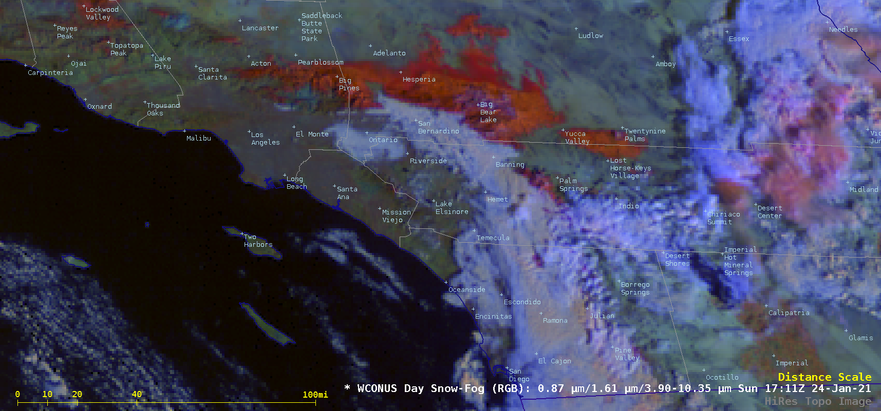
![GOES-17 Day Snow-Fog RGB images [click t play animation | MP4]](https://cimss.ssec.wisc.edu/satellite-blog/images/2021/01/210124_goes17_daySnowFogRGB_SoCal_anim.gif)
![Suomi NPP VIIRS True Color RGB and False Color RGB images [click to enlarge]](https://cimss.ssec.wisc.edu/satellite-blog/images/2021/01/210124_2036utc_suomiNPP_viirs_trueColorRGB_SoCal_anim.gif)


