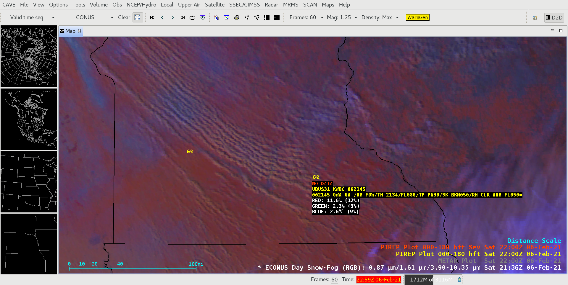
GOES-16 (GOES-East) Day Snow-Fog RGB images (above) showed widespread horizontal convective rolls (HCRs) which highlighted areas where blowing snow was more concentrated across parts of southern Manitoba and the Upper Midwest on 06 February 2021. Snow cover (and glaciated clouds) appeared as shades of red, with bare ground exhibiting lighter shades of green and... Read More
![GOES-16 Day Snow-Fog RGB images [click to play animation | MP4]](https://cimss.ssec.wisc.edu/satellite-blog/images/2021/02/blsn_rgb-20210206_210108.png)
GOES-16 Day Snow-Fog RGB images [click to play animation | MP4]
GOES-16
(GOES-East) Day Snow-Fog RGB images
(above) showed widespread horizontal convective rolls (HCRs) which highlighted areas where blowing snow was more concentrated across parts of southern Manitoba and the Upper Midwest on
06 February 2021. Snow cover (and glaciated clouds) appeared as shades of red, with bare ground exhibiting lighter shades of green and low-level water droplet clouds appearing as brighter shades of white.
Closer views of the northern, central and southern portions of the region where blowing snow was most prevalent are shown below. The HCRs were evident during the early to late morning hours across southern Manitoba, far eastern North Dakota and northwestern Minnesota — and then became more apparent across western/southern Minnesota extending into far northern Iowa as the day progressed. Surface reports showed that the visibility fluctuated dramatically at some sites as HCRs moved through.
![GOES-16 Day Snow-Fog RGB images [click to play animation | MP4]](https://cimss.ssec.wisc.edu/satellite-blog/images/2021/02/blsn1_rgb-20210206_210108.png)
GOES-16 Day Snow-Fog RGB images [click to play animation | MP4]
![GOES-16 Day Snow-Fog RGB images [click to play animation | MP4]](https://cimss.ssec.wisc.edu/satellite-blog/images/2021/02/blsn2_rgb-20210206_210108.png)
GOES-16 Day Snow-Fog RGB images [click to play animation | MP4]
![GOES-16 Day Snow-Fog RGB images [click to play animation | MP4]](https://cimss.ssec.wisc.edu/satellite-blog/images/2021/02/blsn3_rgb-20210206_210108.png)
GOES-16 Day Snow-Fog RGB images [click to play animation | MP4]
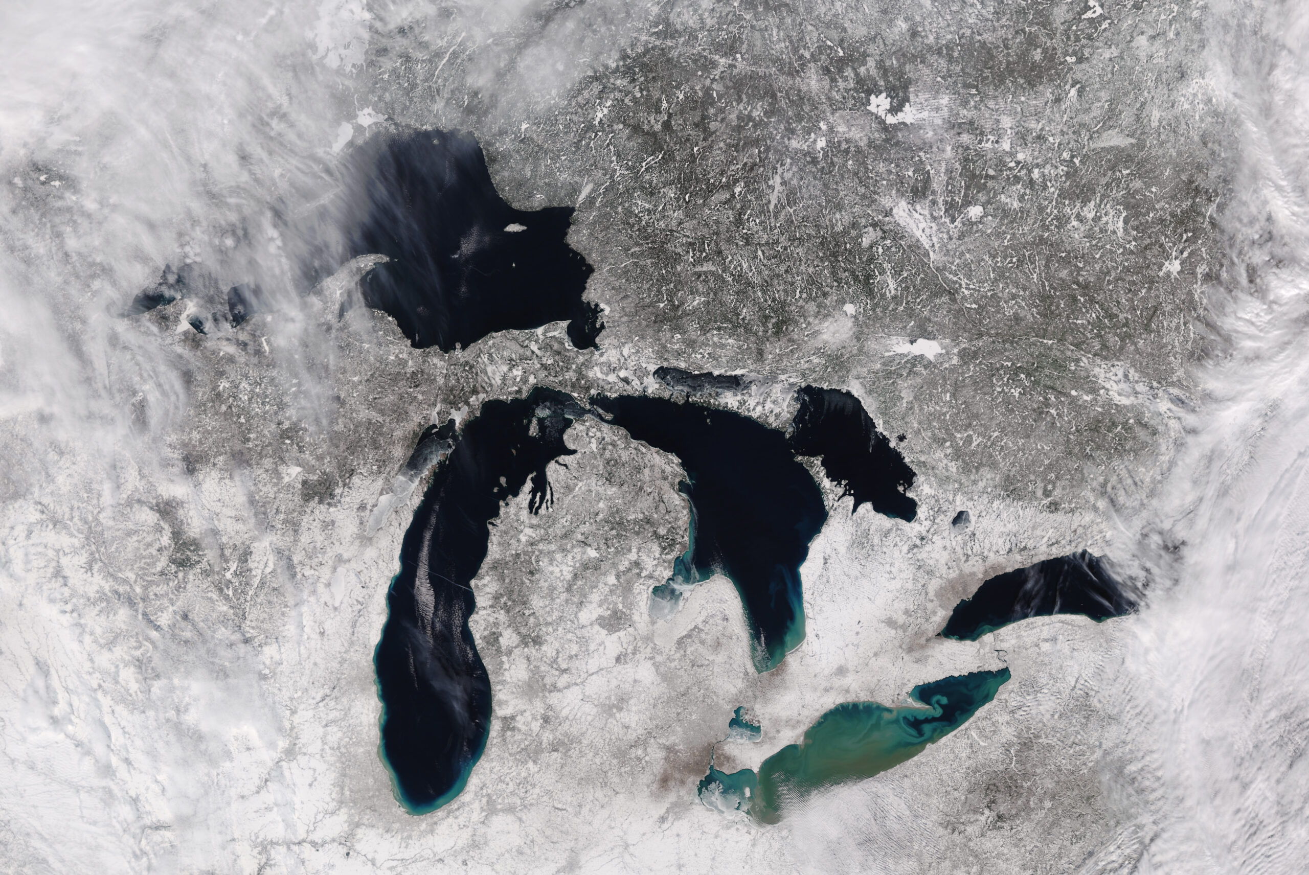
![Terra MODIS True Color and False Color RGB images [click to enlarge]](https://cimss.ssec.wisc.edu/satellite-blog/images/2021/02/210206_1645utc_terra_modis_trueColorRGB_falseColorRGB_Northcentral_US_anim.gif)
Terra MODIS True Color and False Color RGB images [click to enlarge]
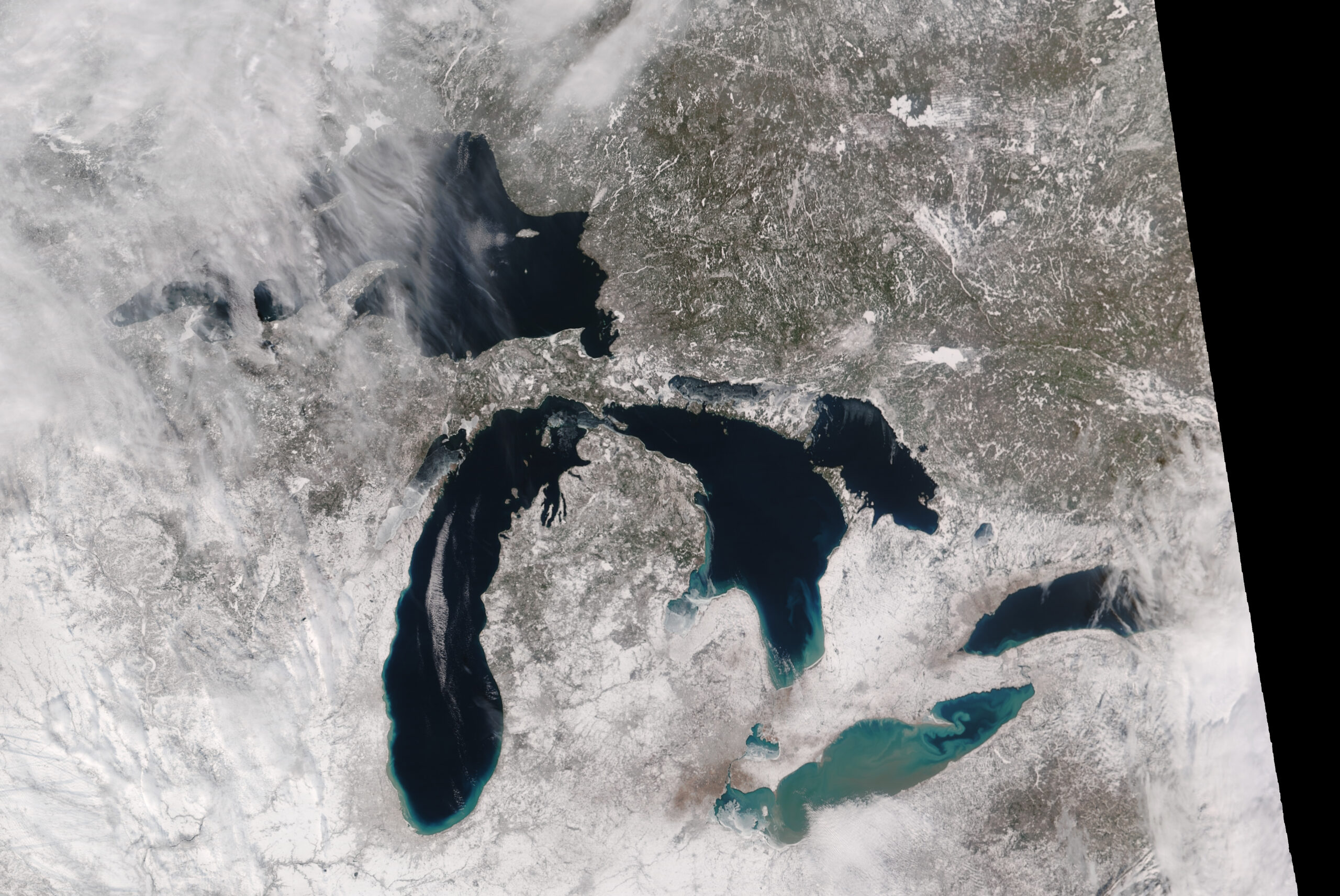
In comparisons of MODIS True Color and False Color RGB images from Terra
(above) and Aqua
(below), the areal coverage of HCRs could be seen in the False Color imagery.
![Aqua MODIS True Color and False Color RGB images [click to enlarge]](https://cimss.ssec.wisc.edu/satellite-blog/images/2021/02/210206_2006utc_aqua_modis_trueColorRGB_falseColorRGB_Northcentral_US_anim.gif)
Aqua MODIS True Color and False Color RGB images [click to enlarge]
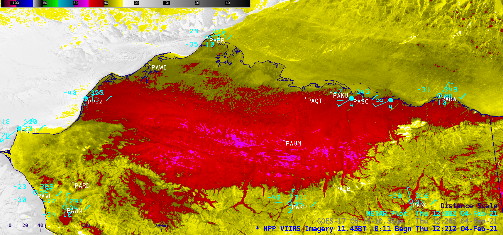
Farthest to the north, one cluster of HCRs appeared to originate over Lake Manitoba — as seen in 30-meter resolution Landsat-8 False Color imagery from
RealEarth (below).
![Landsat-8 False Color RGB image [click to enlarge]](https://cimss.ssec.wisc.edu/satellite-blog/images/2021/02/210206_1712utc_landsat8_falseColorRGB_Manitoba_blowing_snow.png)
Lansdsat-8 False Color RGB image [click to enlarge]
Two notable pilot reports across southern Minnesota
(below) showed that flight visibility was restricted to 4 miles at an elevation of 3000 feet, and the tops of HCRs extended to 5000 feet.
![GOES-16 Day Snow-Fog RGB images, with plots of Pilot Reports [click to enlarge]](https://cimss.ssec.wisc.edu/satellite-blog/images/2021/02/210206_1812utc_pirep.png)
GOES-16 Day Snow-Fog RGB images, with plots of Pilot Reports [click to enlarge]
![GOES-16 Day Snow-Fog RGB images, with plots of Pilot Reports [click to enlarge]](https://cimss.ssec.wisc.edu/satellite-blog/images/2021/02/210206_2134utc_pirep.png)
GOES-16 Day Snow-Fog RGB images, with plots of Pilot Reports [click to enlarge]
Additional material on satellite identification of blowing snow is available
here and
here.
View only this post
Read Less
![GOES-16 Day Snow-Fog RGB images [click to play animation | MP4]](https://cimss.ssec.wisc.edu/satellite-blog/images/2021/02/210206_goes16_daySnowFogRGB_UpperMidwest_blowing_snow_anim.gif)
![GOES-16 Day Snow-Fog RGB images [click to play animation | MP4]](https://cimss.ssec.wisc.edu/satellite-blog/images/2021/02/210206_goes16_daySnowFogRGB_UpperMidwest_blowing_snow_north_anim.gif)
![GOES-16 Day Snow-Fog RGB images [click to play animation | MP4]](https://cimss.ssec.wisc.edu/satellite-blog/images/2021/02/210206_goes16_daySnowFogRGB_UpperMidwest_blowing_snow_central_anim.gif)
![GOES-16 Day Snow-Fog RGB images [click to play animation | MP4]](https://cimss.ssec.wisc.edu/satellite-blog/images/2021/02/210206_goes16_daySnowFogRGB_UpperMidwest_blowing_snow_south_anim.gif)
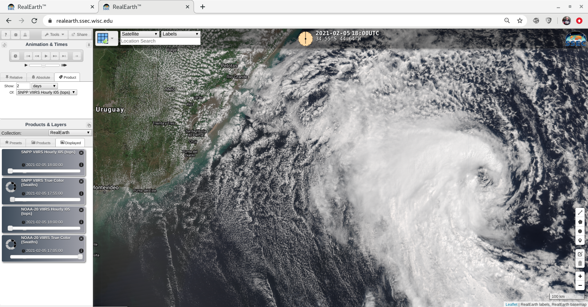
![VIIRS True Color RGB images from Suomi NPP and NOAA-20 [click to enlarge]](https://cimss.ssec.wisc.edu/satellite-blog/images/2021/02/210205_suomiNPP_noaa20_viirs_trueColorRGB_South_Atlantic_cyclone_anim.gif)
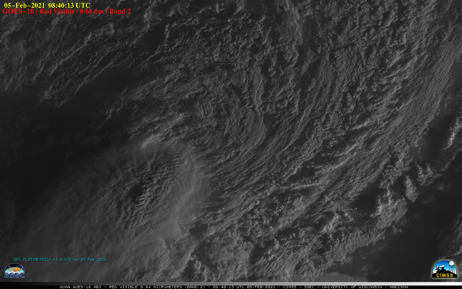
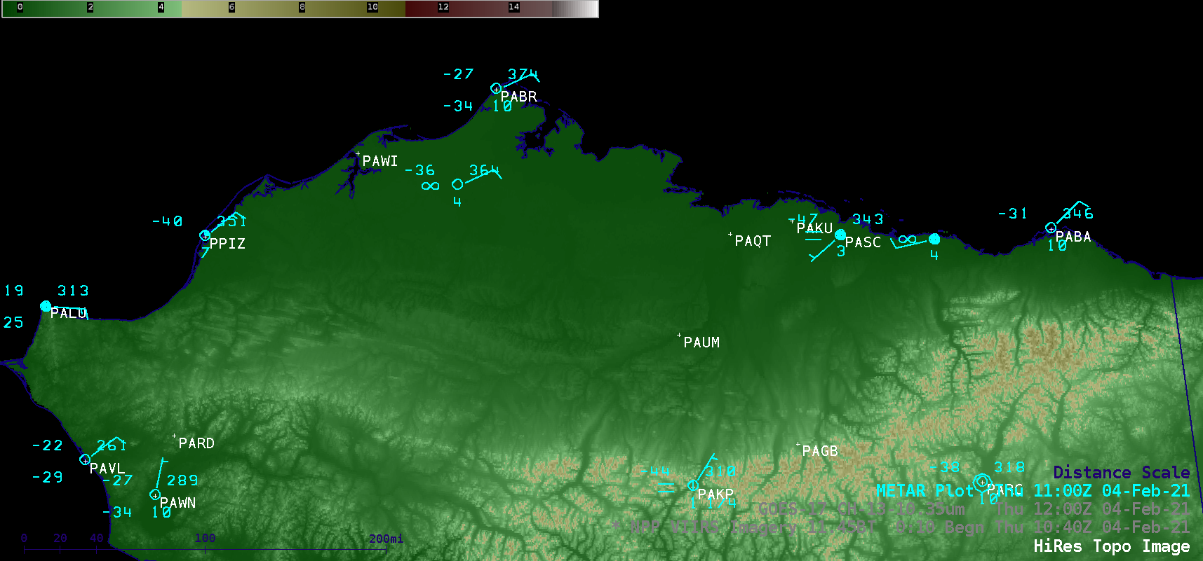
![Suomi NPP VIIRS Infrared Window (11.45 µm) images [click to enlarge]](https://cimss.ssec.wisc.edu/satellite-blog/images/2021/02/210204_suomiNPP_viirs_infrared_AK_anim.gif)
![GOES-17 "Clean" Infrared Window (10.35 µm) images [click to enlarge]](https://cimss.ssec.wisc.edu/satellite-blog/images/2021/02/210204_goes17_infrared_AK_anim.gif)
![Infrared Window images from Suomi NPP VIIRS and GOES-17 (10.35 µm) at 1223 UTC [click to enlarge]](https://cimss.ssec.wisc.edu/satellite-blog/images/2021/02/210204_suomiNPP_goes17_infrared_AK_anim.gif)

