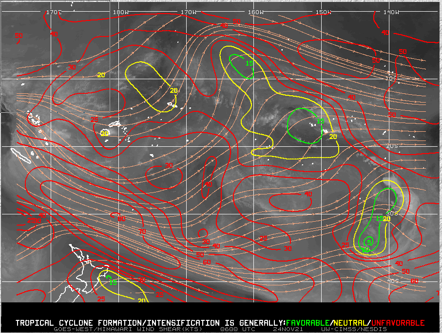
This website works best with a newer web browser such as Chrome, Firefox, Safari or Microsoft Edge. Internet Explorer is not supported by this website.

Severe weather across the Deep South and Mid-South

1-minute Mesoscale Domain Sector GOES-16 “Red” Visible (0.64 µm) images (above) and “Clean” Infrared Window (10.35 µm) images (below) include time-matched plots of SPC Storm Reports that were produced by a number of supercell thunderstorms that developed and moved across the Deep South and Mid-South on 25 March 2021. The highest concentration of tornadoes occurred in Alabama, including one that was responsible for multiple fatalities... Read More

GOES-16 “Red” Visible (0.64 µm) images, with time-matched SPC Storm Reports plotted in red [click to play animation | MP4]

GOES-16 “Red” Visible (0.64 µm) images, with time-matched SPC Storm Reports plotted in red [click to play animation | MP4]

1-minute Mesoscale Domain Sector GOES-16 “Red” Visible (0.64 µm) images (above) and “Clean” Infrared Window (10.35 µm) images (below) include time-matched plots of SPC Storm Reports that were produced by a number of supercell thunderstorms that developed and moved across the Deep South and Mid-South on 25 March 2021. The highest concentration of tornadoes occurred in Alabama, including one that was responsible for multiple fatalities in Ohatchee around 1842 UTC.

GOES-16 “Clean” Infrared Window (10.35 µm) images, with time-matched SPC Storm Reports plotted in cyan [click to play animation | MP4]

GOES-16 “Clean” Infrared Window (10.35 µm) images, with time-matched SPC Storm Reports plotted in cyan [click to play animation | MP4]

In a time-matched comparison of Infrared images from Suomi NPP (overpass times) and GOES-16 at 1831 UTC (below)the coldest overshooting top infrared brightness temperature sensed by the VIIRS instrument on Suomi NPP was -78ºC, compared to -72ºC by the ABI  instrument on GOES-16. Note the small northward parallax displacement that is inherent with GOES-16 imagery over that region. The same color enhancement is applied to both images.

GOES-16 “Clean” Infrared Window (10.35 µm) and Suomi NPP VIIRS Infrared Window (11.45 µm) images at 1921 UTC [click to enlarge]

GOES-16 “Clean” Infrared Window (10.35 µm) and Suomi NPP VIIRS Infrared Window (11.45 µm) images at 1831 UTC [click to enlarge]

View only this post Read Less

Eruption of Mount Etna

EUMETSAT Meteosat-11 Ash Height retrievals from the NOAA/CIMSS Volcanic Cloud Monitoring site (above) showed that an eruption of Mount Etna in Sicily, Italy on 24 March 2021 produced an ash cloud which rose to heights of 7-8 km (darker shade of green).The corresponding Meteosat-11 Ash Loading images are shown below — ash loading... Read More

Meteosat-11 Ash Height images [click to play animation | MP4]

Meteosat-11 Ash Height images [click to play animation | MP4]

EUMETSAT Meteosat-11 Ash Height retrievals from the NOAA/CIMSS Volcanic Cloud Monitoring site (above) showed that an eruption of Mount Etna in Sicily, Italy on 24 March 2021 produced an ash cloud which rose to heights of 7-8 km (darker shade of green).

The corresponding Meteosat-11 Ash Loading images are shown below — ash loading appeared to be light to moderate within much of the volcanic cloud.

Meteosat-11 Ash Loading images [click to play animation | MP4]

Meteosat-11 Ash Loading images [click to play animation | MP4]

Ash Loading values retrieved using Suomi NPP VIIRS data at at 1200 UTC (below) were notably higher than those from Meteosat-11, given the higher spatial resolution and additional spectral band data available from the VIIRS instrument.

Suomi NPP VIIRS Ash Loading at 1200 UTC [click to enlarge]

Suomi NPP VIIRS Ash Loading at 1200 UTC [click to enlarge]

A toggle between VIIRS True Color RGB images from NOAA-20 and Suomi NPP as viewed using RealEarth (below) revealed hues of tan to light brown within the volcanic plume, further supporting the presence of an elevated ash content.

VIIRS True Color RGB images from NOAA-20 and Suomi NPP [click to enlarge]

VIIRS True Color RGB images from NOAA-20 and Suomi NPP [click to enlarge]

View only this post Read Less

Stratus and fog along the US East Coast

GOES-16 (GOES-East) nighttime Cloud Thickness and daytime “Red” Visible (0.64 µm) images (above) displayed a narrow band of marine stratus/fog that was moving southward along the East Coast of the US on 23 March 2021. Plots of Ceiling and Visibility showed that some sites along the coasts of New York, New... Read More

GOES-16 Cloud Thickness and

GOES-16 Cloud Thickness and “Red” Visible (0.64 µm) images, with plots of Ceiling and Visibility [click to play animation | MP4]

GOES-16 (GOES-East) nighttime Cloud Thickness and daytime “Red” Visible (0.64 µm) images (above) displayed a narrow band of marine stratus/fog that was moving southward along the East Coast of the US on 23 March 2021. Plots of Ceiling and Visibility showed that some sites along the coasts of New York, New Jersey and Delaware experienced a reduction in visibility to 1/4 mile at times. The Cloud Thickness product (a component of the Fog/Low Stratus suite) indicated that portions of this feature were 350-400 meters (1150-1300 feet) thick.

With ample illumination from the Moon — which was in the Waxing Gibbous phase, at 68% of Full — a NOAA-20 VIIRS Day/Night Band (0.7 µm) image at 0600 UTC or 2:00 am EDT (below) showed the stratus/fog feature as it was beginning to moved southward along the DelMarVa coast.

NOAA-20 VIIRS Day/Night Band (0.7 ) image [click to enlarge]

NOAA-20 VIIRS Day/Night Band (0.7 µm) image [click to enlarge]

View only this post Read Less

Creating and Displaying gridded GLM fields using data from NOAA CLASS

This blog posts describes how to use NOAA’S CLASS (Comprehensive Large Array-data Stewardship System) system (link) that contains Level-2 GLM data, (under the GOES-R Series GLM L2+ Data Product (GRGLMPROD) tab) to create useable GLM imagery. GLM processing produces three Level 2 files each minute, and those files can be processed to produce imagery. First, choose... Read More

GOES-16 Gridded GLM imagery of Total Optical Energy for the 1 minute ending 1501 UTC on 22 March 2021 (Click to enlarge)

This blog posts describes how to use NOAA’S CLASS (Comprehensive Large Array-data Stewardship System) system (link) that contains Level-2 GLM data, (under the GOES-R Series GLM L2+ Data Product (GRGLMPROD) tab) to create useable GLM imagery. GLM processing produces three Level 2 files each minute, and those files can be processed to produce imagery. First, choose the time range you want in CLASS, and get the global imagery.  For this blog post, I chose GOES-16 data on 22 March 2021 between 15:00 an 15:15 UTC.  On the CLASS website, I clicked the GLM L2+ Lightning Detection Data and didn’t filter by any values (CLASS allows you to filter by minimum/maximum flash, event and group counts, if you want).  This request returned 47 different files, but that is only about 10 Mbytes.  Some of the file names — two minutes’ worth — are shown below: LCFA files from julian Day 081 (that is, 3/22/2021) starting at 15:00:00:00, 15:00:00:20, 15:00:00:40, … etc.


OR_GLM-L2-LCFA_G16_s20210811500000_e20210811500203_c20210811500218.nc
OR_GLM-L2-LCFA_G16_s20210811500200_e20210811500404_c20210811500425.nc
OR_GLM-L2-LCFA_G16_s20210811500400_e20210811501003_c20210811501016.nc
OR_GLM-L2-LCFA_G16_s20210811501000_e20210811501205_c20210811501226.nc
OR_GLM-L2-LCFA_G16_s20210811501200_e20210811501403_c20210811501419.nc

Code to convert these files (that contain raw-ish group, event and flash fields) to gridded GLM fields (that can be displayed with, for example, Geo2Grid, or AWIPS) is within the CSPP Gridded GLM software package that can be downloaded here (free registration may be required; the Gridded GLM tarball to download includes a short and useful README). To create a data file that is properly configured for Geo2Grid (or AWIPS), with software that uses the open-source glmtools software developed by Dr. Eric Bruning at Texas Tech, use this command:

cspp-geo-gglm.sh ../../data/OR_GLM-L2-LCFA_G16_s20210811501*

That will create a file with a name like this:

CG_GLM-L2-GLMF-M3_G16_s20210811501000_e20210811502000_c20210821745120.nc;

Geo2Grid can then be used to create imagery from the newly-created netCDF file. The Geo2Grid code used is below.

../p2g_grid_helper.sh TestGridded -75.0 8. 1000 -1000 2000 750 > $GEO2GRID_HOME/TestGridded.conf
../geo2grid.sh -r glm_l2 -w geotiff -p total_energy -g TestGridded --grid-configs $GEO2GRID_HOME/TestGridded.conf --method nearest -f /home/scottl/CSPPGeo/GGLM/cspp-geo-gridded-glm-1.0b1/bin/CG_GLM-L2-GLMF-M3_G16_s20210811501000_e20210811502000_c20210821745120.nc
../add_colormap.sh ../../../enhancements/TotalEnergy.txt GOES-16_GLM_total_energy_20210322_150100_TestGridded.tif
../add_coastlines.sh --add-coastlines --coastlines-resolution=h --coastlines-outline='black' --add-grid --grid-text-size 12 --grid-d 1.0 1.0 --grid-D 1.0 1.0 --add-colorbar --colorbar-tick-marks 250.0 --colorbar-text-size 1 --colorbar-no-ticks --colorbar-align bottom GOES-16_GLM_total_energy_20210322_150100_TestGridded.tif
convert GOES-16_GLM_total_energy_20210322_150100_TestGridded.png -gravity Southwest -fill white -pointsize 24 -annotate +8+30 "1501 UTC 22 March 2021 Total Energy" GOES-16_GLM_total_energy_20210322_1501_Labeled.png

The Geo2Grid package commands above (1) created the grid (‘TestGridded’) onto which the data were interpolated; (2) created the imagery from the netCDF file output from the Gridded GLM package; (3) Added a pre-defined colormap (within ‘TotalEnergy.txt’); (4) Added coastlines, a lat/lon grid, and a colorbar and (5) annotated the image. This last command used ImageMagick.

Note that the GLM image created, shown at top, is mostly transparent. Three areas of GLM observations are apparent, two over South America, one over the Pacific Ocean south of Panama. The transparency is handy if you want to overlay GLM data on top of ABI imagery!

View only this post Read Less