This website works best with a newer web browser such as Chrome, Firefox, Safari or Microsoft
Edge. Internet Explorer is not supported by this website.
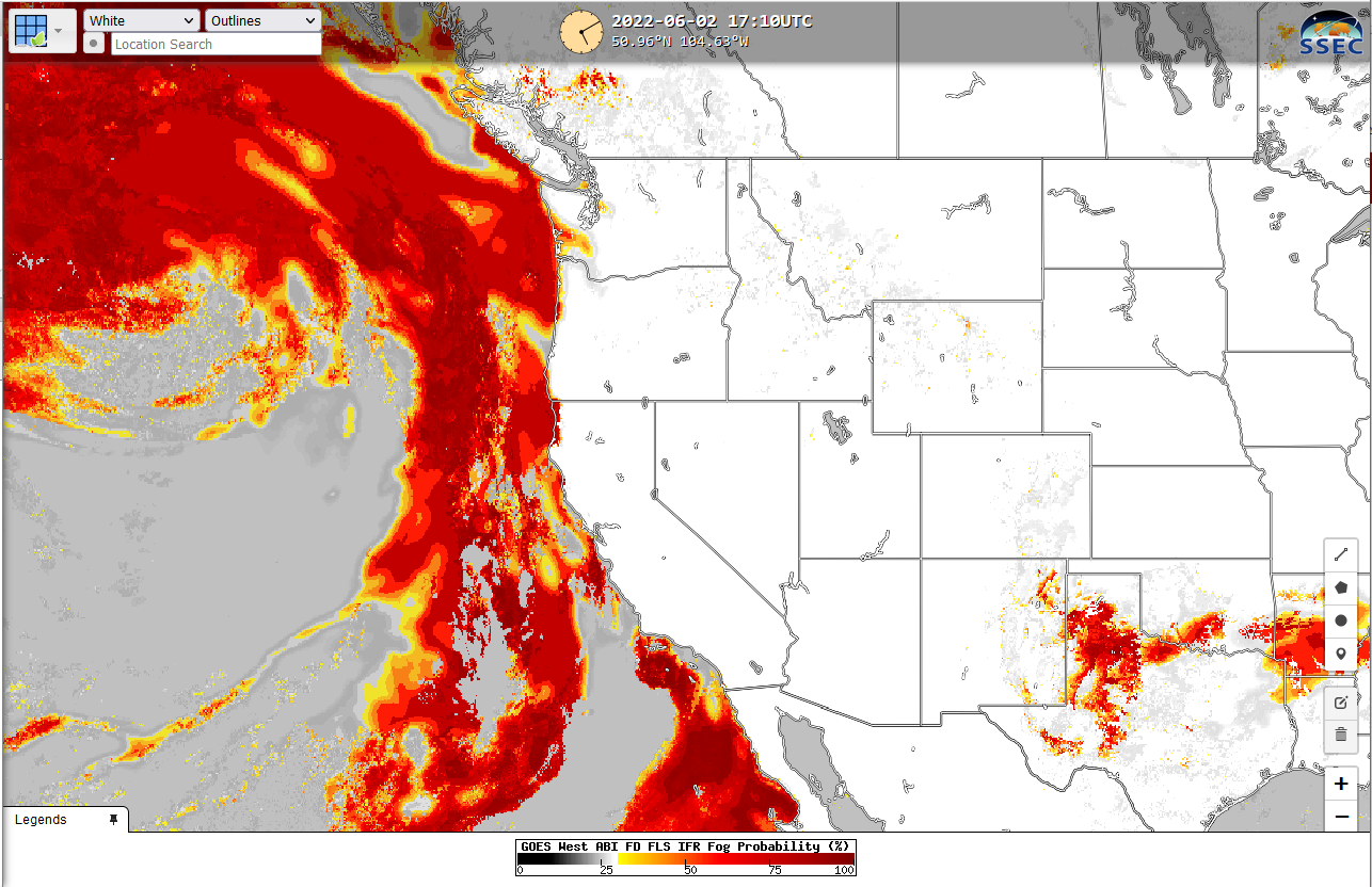
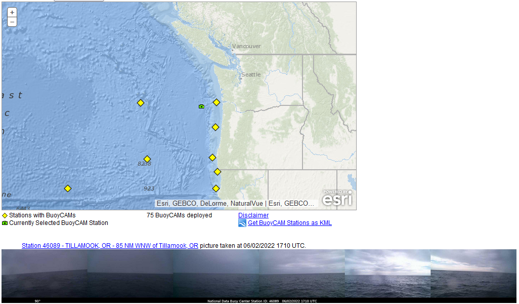
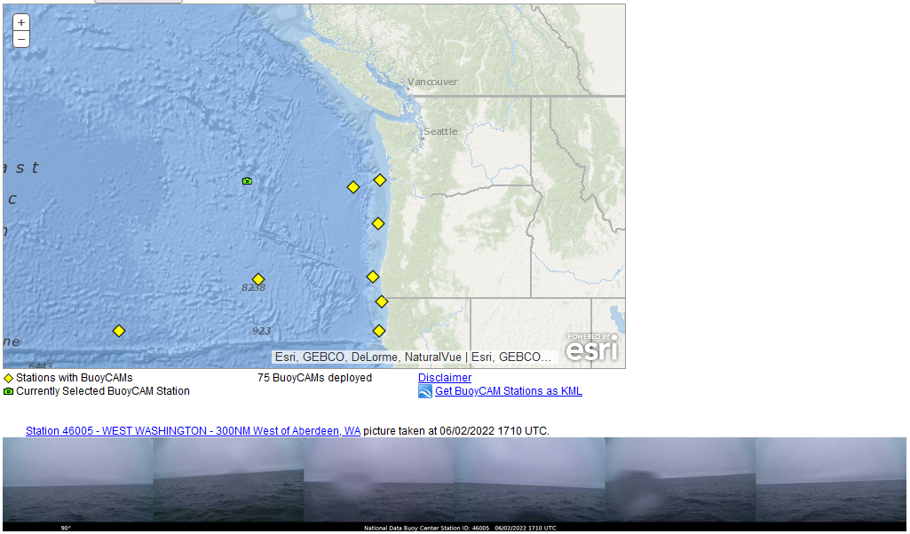
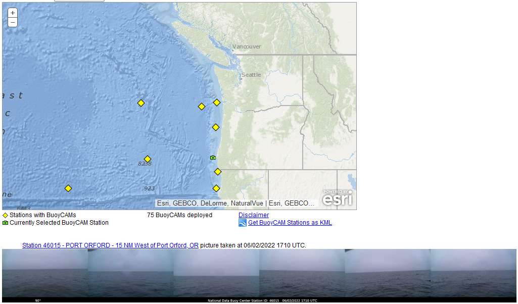
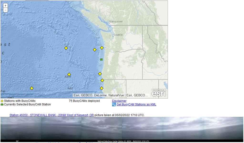
Some National Data Buoy Center buoys do include webcams that provide sky information (link). How well do those observations compare to IFR Probability fields, as shown above in an image from RealEarth? There are three BuoyCams along the Oregon coastline, as shown in the image below, and 3 more offshore... Read More
GOES-17 IFR Probability fields, 1710 UTC on 2 June 2022 (click to enlarge)
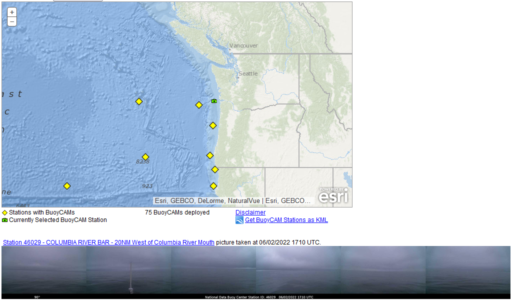
Some National Data Buoy Center buoys do include webcams that provide sky information (link). How well do those observations compare to IFR Probability fields, as shown above in an image from RealEarth? There are three BuoyCams along the Oregon coastline, as shown in the image below, and 3 more offshore that can be compared to the IFR Probability fields above. Consider Buoy 46029, 20 nm offshore of the mouth of the Columbia River, shown below. It shows what appear to be low overcast skies in a region where IFR Probabilities are large. Proceed counterclockwise around the 6 buoys near/offshore Oregon (the one just south of the Oregon/California border is not included here), and you’ll note low clouds are present in most of the BuoyCam observations: Buoy 46089; Buoy 46005; Buoy 46002; Buoy 46015. Only Buoy 46050, along the central Oregon coast, shows multiple breaks in the clouds. This is in a region where IFR Probabilities are smaller!
Webcam observations from Buoy 46029, 1710 UTC on 2 June 2022. Note that the left-most webcam view points towards 90o. (Click to enlarge)
The animation below shows the 6 WebCam observations in sequence. Use these webcams to become more confident in using IFR Probability fields in the open ocean.
Webcam views at 1710 UTC near and offshore from the Oregon Coast (Click to enlarge)
The mp4 animation above (produced using CSPP Geosphere‘s latest beta version) shows strong convection over Oklahoma and the eastern Texas panhandle, with lower clouds (in a bluish hue) over the northwestern Texas panhandle. With time, the Night Microphysics RGB acquires a reddish hue (as cloud tops cool), and then convection develops.... Read More
GOES-16 Night Microphysics RGB, 0701-0911 UTC on 1 June 2022
The mp4 animation above (produced using CSPP Geosphere‘s latest beta version) shows strong convection over Oklahoma and the eastern Texas panhandle, with lower clouds (in a bluish hue) over the northwestern Texas panhandle. With time, the Night Microphysics RGB acquires a reddish hue (as cloud tops cool), and then convection develops. A nowcaster can use changes in the colors of this RGB to anticipate initiation. (A similar recent example is shown here).
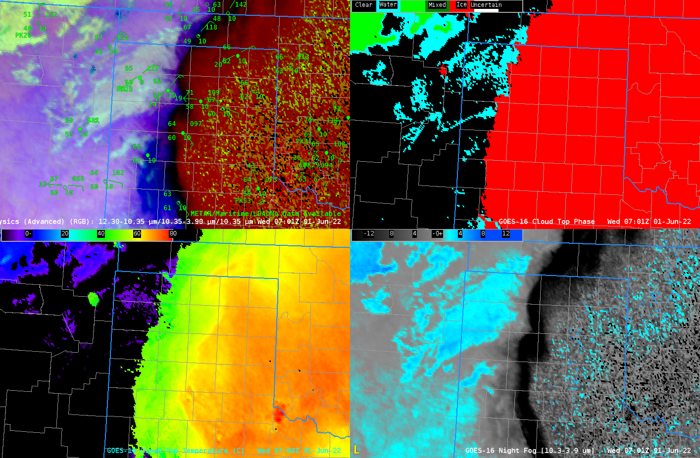
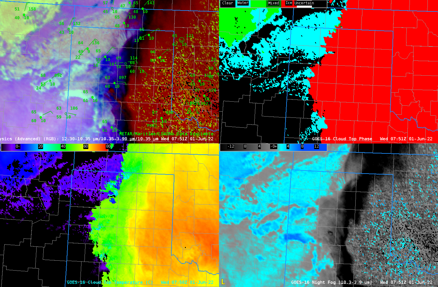
The AWIPS imagery from 0701 UTC below shows the RGB with Level 2 Products: Cloud Top Phase — showing liquid water clouds over Texas where the RGB suggests low clouds, and Cloud Top Temperature — where values of 7-8oC are common. The default color table Cloud Top Temperature has been changed. Recall also that the Level 2 Cloud Top Temperature product is not produced for the CONUS sector, so Full-Disk values are shown. Surface winds suggest low-level convergence: winds are northeasterly over the NW Texas panhandle, and southeasterly to easterly over the southern portions of the Texas panhandle. GOES-16 Cloud Top Heights (not shown) show cloud heights around 12000 feet over the NW Texas panhandle.
GOES-16 Night Microphysics RGB (along with surface observations) (upper left); GOES-16 Cloud Top Phase (Upper right); GOES-16 Cloud-Top Temperature (lower left); GOES-16 Night Fog Brightness Temperature Difference (Lower right). All at 0701 UTC on 1 June 2022 (click to enlarge)
Fifty minutes later, at 0751, the band of low clouds over the northeastern Texas panhandle has reddened somewhat (click here for a toggle between 0701 and 0751). Cloud top temperatures in that cloud band have dropped to between 1o and 4oC, and cloud top heights have increased to 14000 feet. Cloud-top phase is still liquid however (except over northern New Mexico, as might be inferred by the yellower tinge to those low clouds in the RGB). There is also a red tint to the RGB just north of the obvious east-west band of clouds near the Hereford TX airport (where the temperature and dewpoint are 65 and 60, respectively, and no wind is reported). Convective initiation is likely occurring in these regions.
GOES-16 Night Microphysics RGB (along with surface observations) (upper left); GOES-16 Cloud Top Phase (Upper right); GOES-16 Cloud-Top Temperature (lower left); GOES-16 Night Fog Brightness Temperature Difference (Lower right). All at 0751 UTC on 1 June 2022 (click to enlarge)
From 0801 to 0816 UTC, shown below, supercooled clouds are noted, as the Night Microphysics RGB continues to redden. By 0816 UTC, mixed phase clouds are noted in the line developing near Hereford. Cloud-top heights increase from 15000 to 21000 feet between 0811 and 0816 UTC.
GOES-16 Night Microphysics RGB (along with surface observations) (upper left); GOES-16 Cloud Top Phase (Upper right); GOES-16 Cloud-Top Temperature (lower left); GOES-16 Night Fog Brightness Temperature Difference (Lower right). 0801-0816 on 1 June 2022 (click to enlarge)
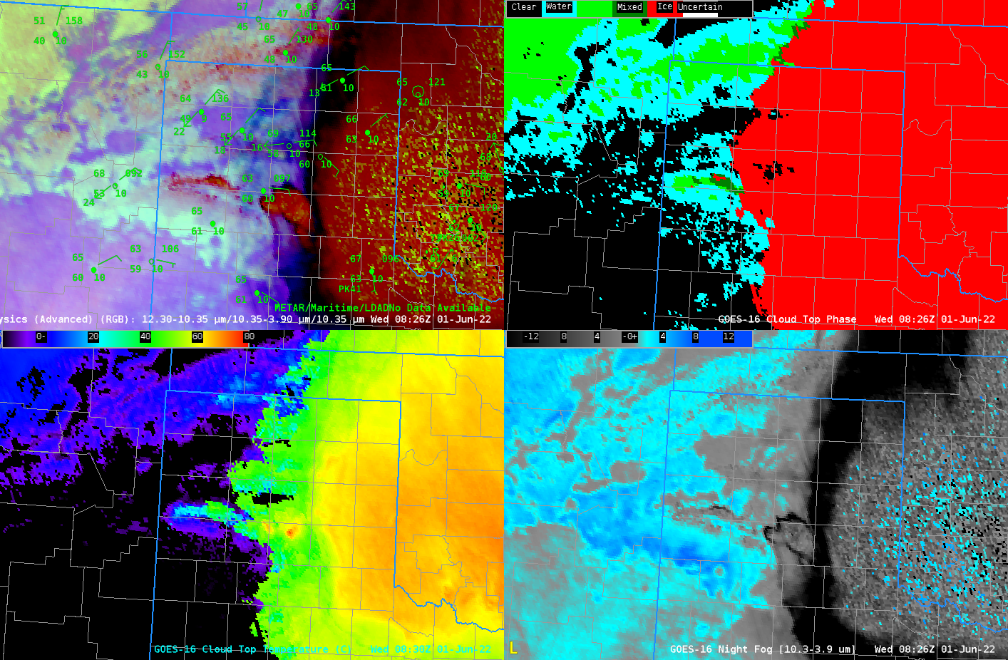
By 0826 UTC, Cloud Tops are shown to include ice over the line developing over the east-central part of the Texas panhandle.
GOES-16 Night Microphysics RGB (along with surface observations) (upper left); GOES-16 Cloud Top Phase (Upper right); GOES-16 Cloud-Top Temperature (lower left); GOES-16 Night Fog Brightness Temperature Difference (Lower right). All at 0826 UTC on 1 June 2022 (click to enlarge)
A rocking animation of the 4-panels above, from 0801 to 0901 (and back) is here. If convection is expected overnight, and low clouds are present, use the Night Time Microphysics RGB to monitor when convection might initiate. Color changes in the low clouds give important information.
1-minute Mesoscale Domain Sector GOES-16 (GOES-East) “Red” Visible (0.64 µm) images (above) include time-matched SPC Storm Reports — and showed the development severe thunderstorms across parts of the Upper Midwest during the afternoon and early evening hours on 30 May 2022. These storms produced several tornadoes, hail as large as 2.00 inches in diameter and damaging winds as strong as... Read More
GOES-16 “Red” Visible (0.64 µm) images, with time-matched SPC Storm Reports plotted in red [click to play animated GIF | MP4]
1-minute Mesoscale Domain Sector GOES-16 (GOES-East) “Red” Visible (0.64 µm) images (above) include time-matched SPC Storm Reports — and showed the development severe thunderstorms across parts of the Upper Midwest during the afternoon and early evening hours on 30 May 2022. These storms produced several tornadoes, hail as large as 2.00 inches in diameter and damaging winds as strong as 90 mph.
In the corresponding 1-minute GOES-16 “Clean” Infrared Window (10.35 µm) images (below), pulsing overshooting tops exhibited infrared brightness temperatures as cold as -70ºC (darker black enhancement).
GOES-16 “Clean” Infrared Window (10.35 µm) images, with time-matched SPC Storm Reports plotted in blue [click to play animated GIF | MP4]
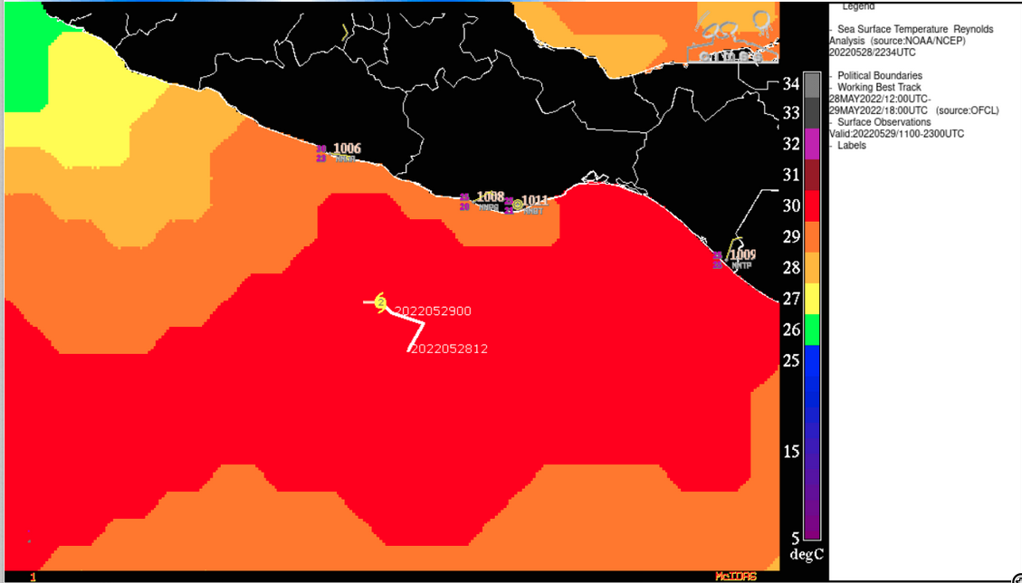
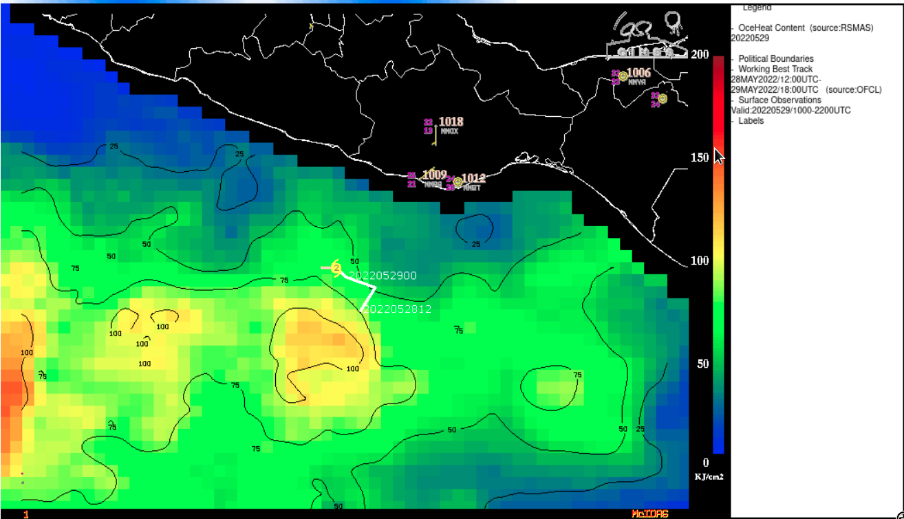
1-minute Mesoscale Domain Sector GOES-17 (GOES-West) — and GOES-16 (GOES-East) after 1621 UTC — “Clean” Infrared Window (10.35 µm) and “Red” Visible (0.64 µm) images (above) showed Hurricane Agatha after the tropical storm reached hurricane intensity at 1200 UTC on 29 May 2022. Overshooting tops near the storm center exhibited infrared brightness temperatures... Read More
GOES-17 and GOES-16 “Clean” Infrared Window (10.35 µm) and “Red” Visible (0.64 µm) images [click to play animated GIF | MP4]
1-minute Mesoscale Domain Sector GOES-17 (GOES-West) — and GOES-16 (GOES-East) after 1621 UTC — “Clean” Infrared Window (10.35 µm) and “Red” Visible (0.64 µm) images (above) showed Hurricane Agatha after the tropical storm reached hurricane intensity at 1200 UTC on 29 May 2022. Overshooting tops near the storm center exhibited infrared brightness temperatures as cold as -90 to -95ºC at times.
GOES-16 Infrared Window (11.2 µm) images from the CIMSS Tropical Cyclones site (below) include contours of deep-layer wind shear at 12 UTC and 21 UTC — which indicated that Agatha was moving through an environment of relatively low shear, one factor that favored its phase of rapid intensification (ADT | SATCON).
GOES-16 Infrared Window (11.2 µm) images, with contours of deep-layer wind shear at 12 UTC [click to enlarge]
GOES-16 Infrared Window (11.2 µm) images, with contours of deep-layer wind shear at 21 UTC [click to enlarge]
GOES-16 “Red” Visible (0.64 µm, left) and “Clean” Infrared Window (10.35 µm, right) images [click to play animated GIF | MP4]
Hurricane Agatha made landfall along the southern coast of Mexico — between Puerto Escondido MMPS and Bohias De Huatulco MMBT — around 2040 UTC on 30 May, as seen in 1-minute GOES-16 Visible and Infrared images (above).


