This website works best with a newer web browser such as Chrome, Firefox, Safari or Microsoft
Edge. Internet Explorer is not supported by this website.
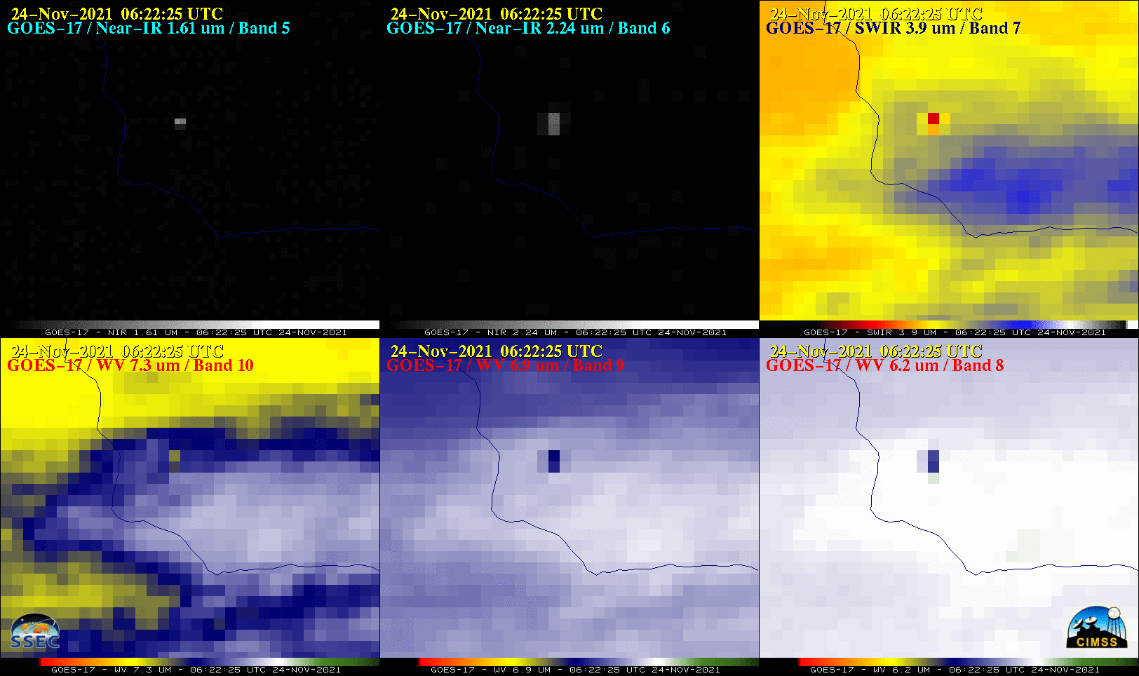
1-minute Mesoscale Domain Sector GOES-17 (GOES-West) Near-Infrared “Snow/Ice” (1.61 µm). Near-Infrared “Cloud Particle Size” (2.24 µm), Shortwave Infrared (3.9 µm), Low-level (7.3 µm). Mid-level (6.9 µm) and Upper-level (6.2 µm) Water Vapor images (above) showed signatures of the DART Mission from Vandenberg Space Force Base in southern California on 24 November 2021. Shortly after the 0620 UTC launch, a warm thermal... Read More
GOES-17 Near-Infrared, Shortwave Infrared and Water Vapor images [click to play animated GIF | MP4]
1-minute Mesoscale Domain Sector GOES-17 (GOES-West) Near-Infrared “Snow/Ice” (1.61 µm). Near-Infrared “Cloud Particle Size” (2.24 µm), Shortwave Infrared (3.9 µm), Low-level (7.3 µm). Mid-level (6.9 µm) and Upper-level (6.2 µm) Water Vapor images (above) showed signatures of the DART Mission from Vandenberg Space Force Base in southern California on 24 November 2021. Shortly after the 0620 UTC launch, a warm thermal signature of the SpaceX Falcon 9 booster appeared in all 6 of these ABI spectral bands. Note that there were two 0621 UTC images; the 06:21:17 image was from the GOES-17 CONUS Sector — which, because it was scanning a much larger area, didn’t actually scan the rocket plume until around 06:21:57 UTC (the GOES-17 Mesoscale Sector 1 was scanning the rocket plume about 2 seconds earlier, at 06:21:55 UTC).
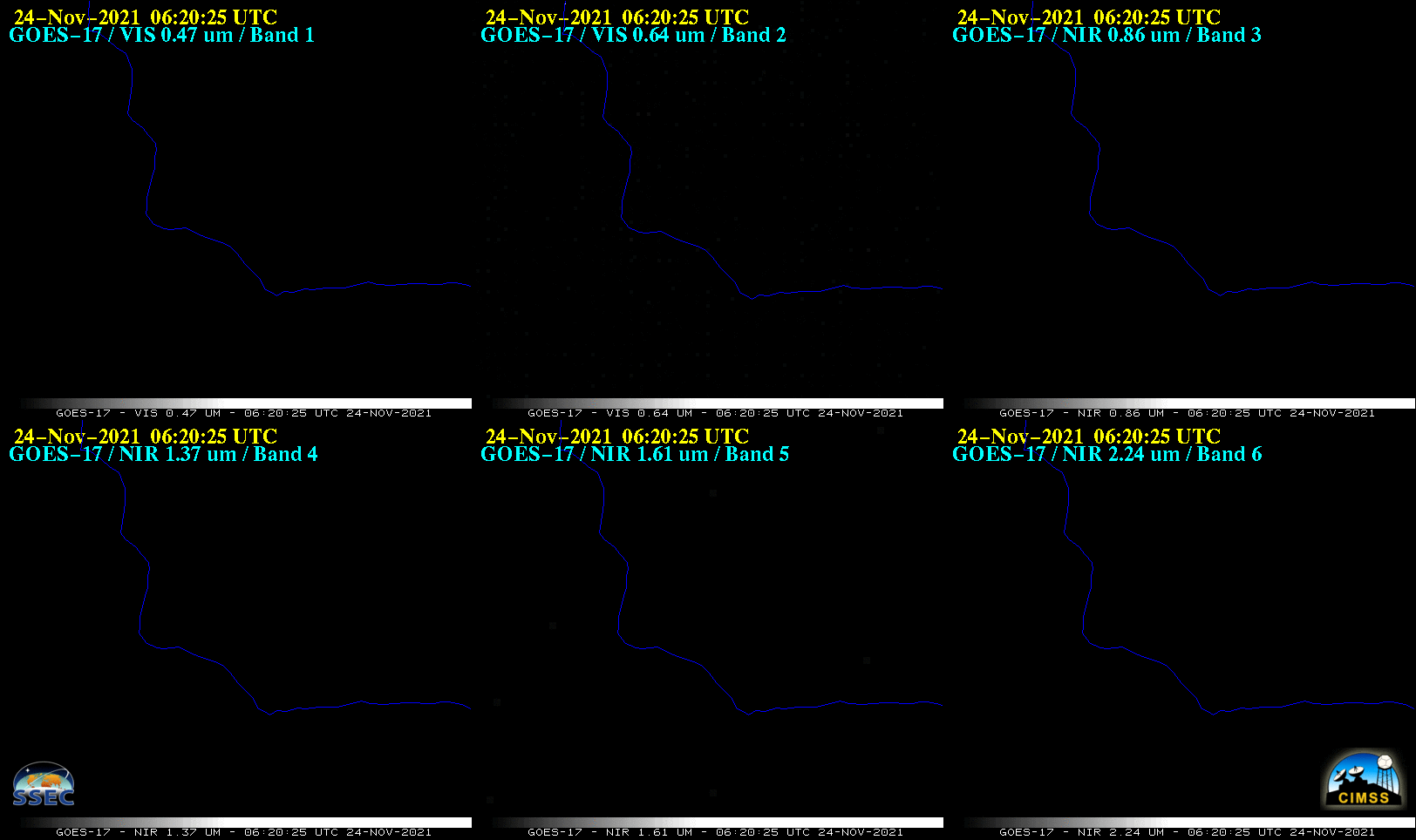
The corresponding GOES-17 Visible (spectral bands 1 and 2) and Near-Infrared (spectral bands 3-6) images are shown below. Since the satellite was viewing the rocket from the west, a very faint reflectance signature of the Falcon 9 booster could be seen in the first 3 post-launch 0.64 µm (Band 2) Visible images — but no discernible signature was evident in the lower-resolution 0.47 µm (Band 1) Visible imagery.
GOES-17 Visible and Near-Infrared images [click to play animated GIF | MP4]
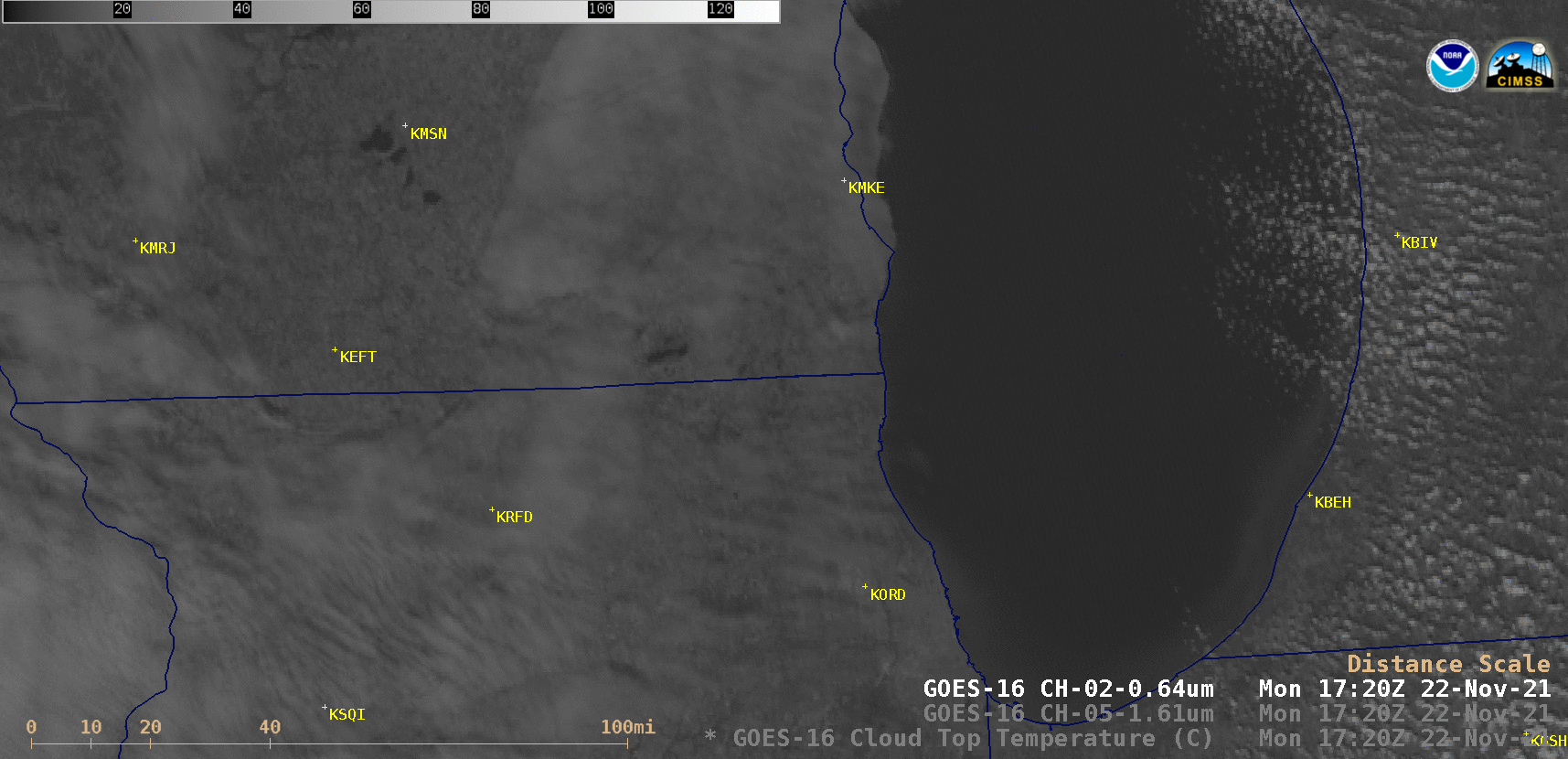
GOES-16 (GOES-East) “Red” Visible (0.64 µm) and Near-Infrared “Snow/Ice” (1.61 µm) images (above) revealed the formation of several “hole punch” features across southeastern Wisconsin, northeastern Illinois and Lake Michigan on 22 November 2021 . These cloud features were caused by aircraft that were either ascending or descending through a relatively thin layer of clouds... Read More
GOES-16 “Red” Visible (0.64 µm) and Near-Infrared “Snow/Ice” (1.61 µm) images [click to play animated GIF | MP4]
GOES-16 (GOES-East) “Red” Visible (0.64 µm) and Near-Infrared “Snow/Ice” (1.61 µm) images (above) revealed the formation of several “hole punch” features across southeastern Wisconsin, northeastern Illinois and Lake Michigan on 22 November 2021 . These cloud features were caused by aircraft that were either ascending or descending through a relatively thin layer of clouds composed of supercooled water droplets — cooling from wake turbulence (reference) and/or particles from the jet engine exhaust acted as ice condensation nuclei, causing the small supercooled water droplets to turn into larger ice crystals (many of which then fall from the cloud layer, creating “fallstreak holes“). The ice crystal clouds appear as darker shades of gray on the 1.61 µm Snow/Ice images.
The GOES-16 Cloud Top Temperature derived product (below) showed that values were generally in the -30 to -35ºC range.
GOES-16 Cloud Top Temperature product [click to play animated GIF | MP4]
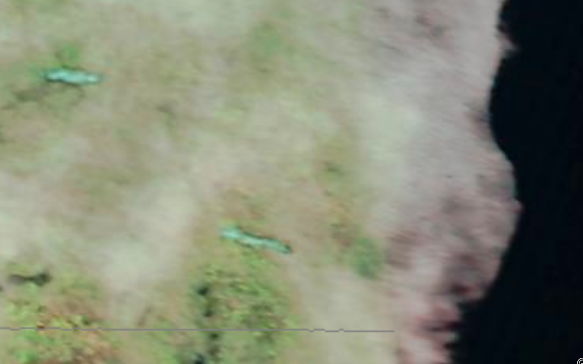
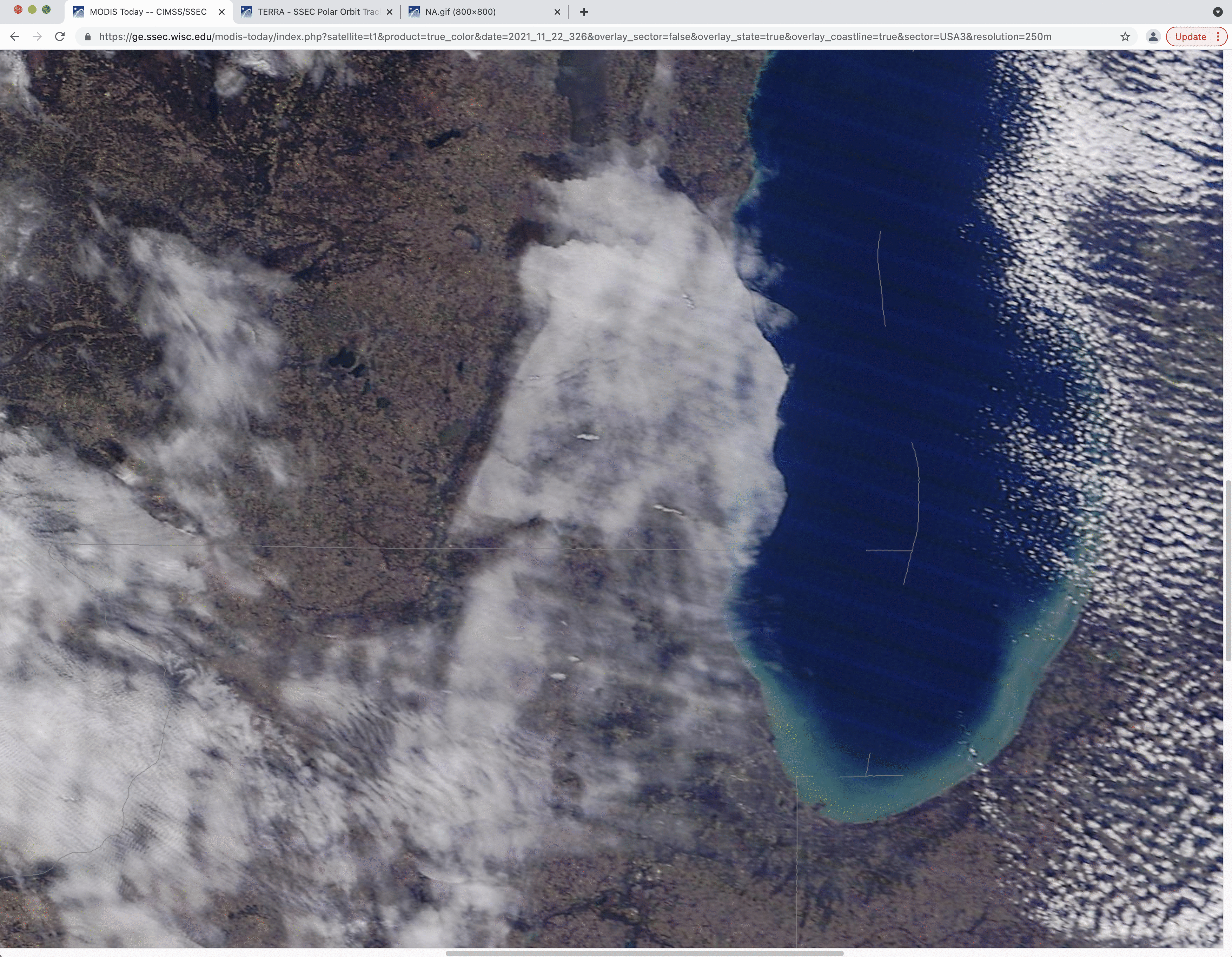
A toggle between 250-meter resolution Terra MODIS True Color and False Color RGB images from the MODIS Today site (below) provided a more detailed view of the numerous hole punch features at 1730 UTC, including a better depiction of the glaciated fallstreak clouds (shades of cyan) within the middle of each hole punch.
Terra MODIS True Color and False Color RGB images [click to enlarge]
Other blog posts showing examples of hole punch features can be found at thislink.
From an email came this question: RADARSAT vs ASCAT winds, what are the differences between the two methods?This comparison is not easy to make directly, as the orbits of Metop-B and Metop-C, the two satellites that carry the ASCAT instrument (now that Metop-A, which satellite also carried ASCAT, has been decomissioned), don’t... Read More
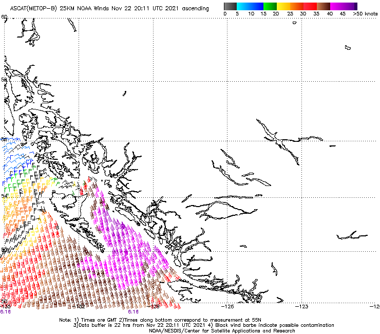
ASCAT winds from Metop-B, 0616 and 1826 on 22 November 2021 (Click to enlarge)
From an email came this question: RADARSAT vs ASCAT winds, what are the differences between the two methods?
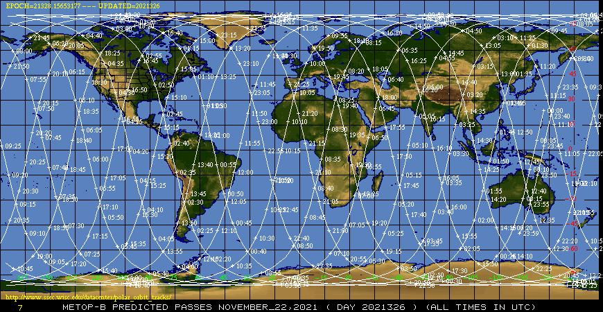
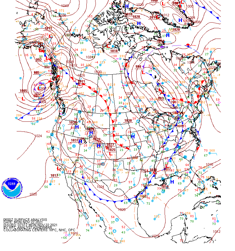
This comparison is not easy to make directly, as the orbits of Metop-B and Metop-C, the two satellites that carry the ASCAT instrument (now that Metop-A, which satellite also carried ASCAT, has been decomissioned), don’t sample the ocean at the same time/location as RADARSAT. The toggle above shows ASCAT winds from Metop-B (Metop-B orbits on 22 November 2021 are here, from this website) at 0631 and 1826 UTC on 22 November (from this source) in the region around Haida Gwaii (once known as the Queen Charlotte Islands). An obvious frontal passage occurred between those two times; this is also shown in the animation of surface charts (every 3 hours from 0600 through 1500 UTC shown here).
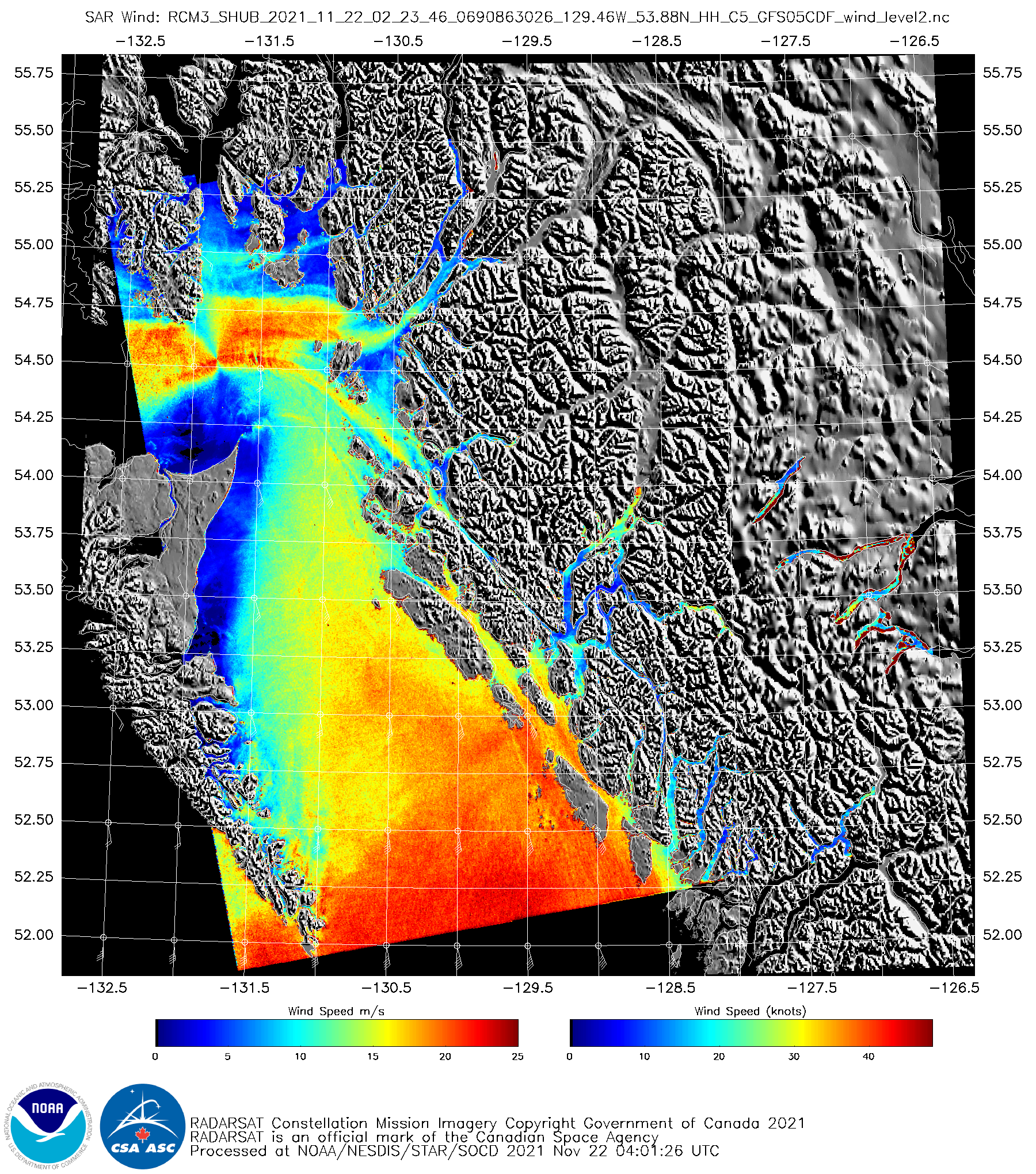
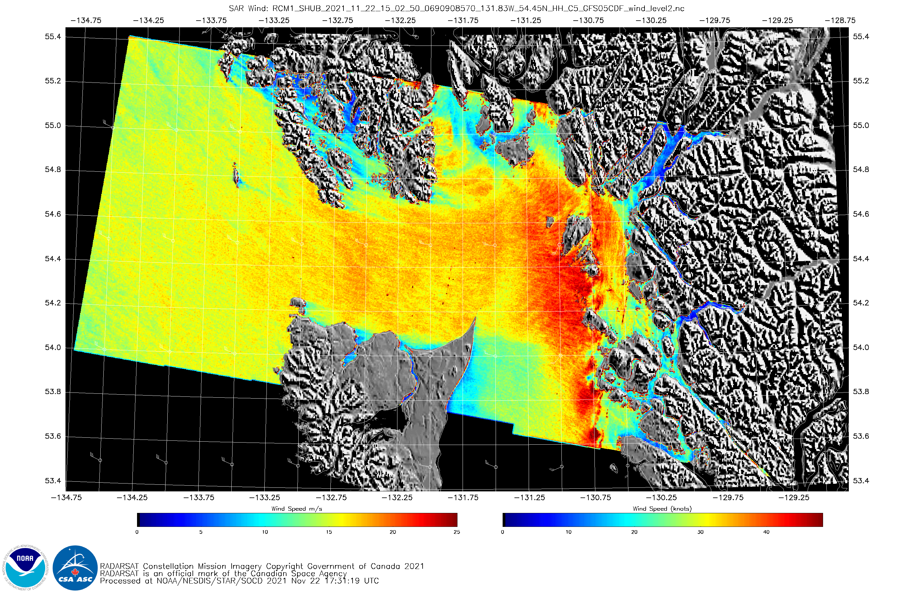
Imagery below shows SAR winds from RCM3 and RCM1 (RCM = RADARSAT Constellation Mission) at 02:23 (top) and around 15:03 (bottom) UTC on 22 November. The 15:03:52 image that follows the two images at bottom is here.
RCM3 RADARSAT SAR winds at 02:23 UTC on 22 November 2021 (Click to enlarge)RCM1 RADARSAT SAR winds, 15:02:50 – 15:03:13 on 22 November 2021 (Click to enlarge)
How does scatterometery measure winds? If wind speeds over the ocean (or a lake) are very light, the water surface will be smooth. Microwave energy from a side-looking radar (ASCAT and SAR are both active radars; that is, they emit a ping and listen for a response) will reflect off it, and not scatter back to the instrument. As winds increase, small ripples develop and backscatter increases. Backscattered energy is greatest if the radar look and the wind direction are aligned; also, the backscatter is greater if the wind is blowing towards (vs. away from) the satellite. This is a source of ambiguity in direction. The backscatter distribution sensed has a name: Normalized Radar Cross-Section (NRCS); many different wind speed/direction combinations can produce the same NRCS. How can you mitigate these ambiguities?
For ASCAT instruments, the ambiguity is reduced through multiple measurements of the same surface — this gives NRCS values with different aspect and incident angles. Multiple measurements are achieved via the multiple antennas that are part of the ASCAT instrument (similarly, rotating beams on instruments such as AMSR-2 give multiple observations). Multiple observations allow for an accurate estimate of wind direction given the observations.
SAR processing mitigates the ambiguities by using numerical model output that suggests the correct wind direction. A challenge is that numerical model data has a far coarser resolution than SAR data. (Model data might also include errors!) As a result, artifacts can be introduced, and a good example is shown in the 02:23 UTC image above at 54.6 N, 131.8 W. In that region, where the windspeeds have an hourglass shape, the model wind direction is unlikely to be consistent with the observations. Keep that in mind when observing SAR winds.
One other aspect of the ASCAT v. SAR wind comparison bears notice: ASCAT winds have a typical upper bound, at around 45-50 knots. At stronger wind speeds, the backscatter to the ASCAT instrument is affected by foam on the sea surface that typically accompanies such strong winds. Special SAR wind processing (as discussed here) allows for observations of much stronger winds, as shown for 2020’s Hurricane Laura, where Seninel-1 SAR observations peaked at 150 knots! These computations use cross-polarization observations from SAR. Both SAR and ASCAT use co-polarization observations. Future ASCAT missions will support cross-polarization observations.
Some of the information above came from this link (specifically, here). If there are errors in the description, they’re this blogger’s fault however.
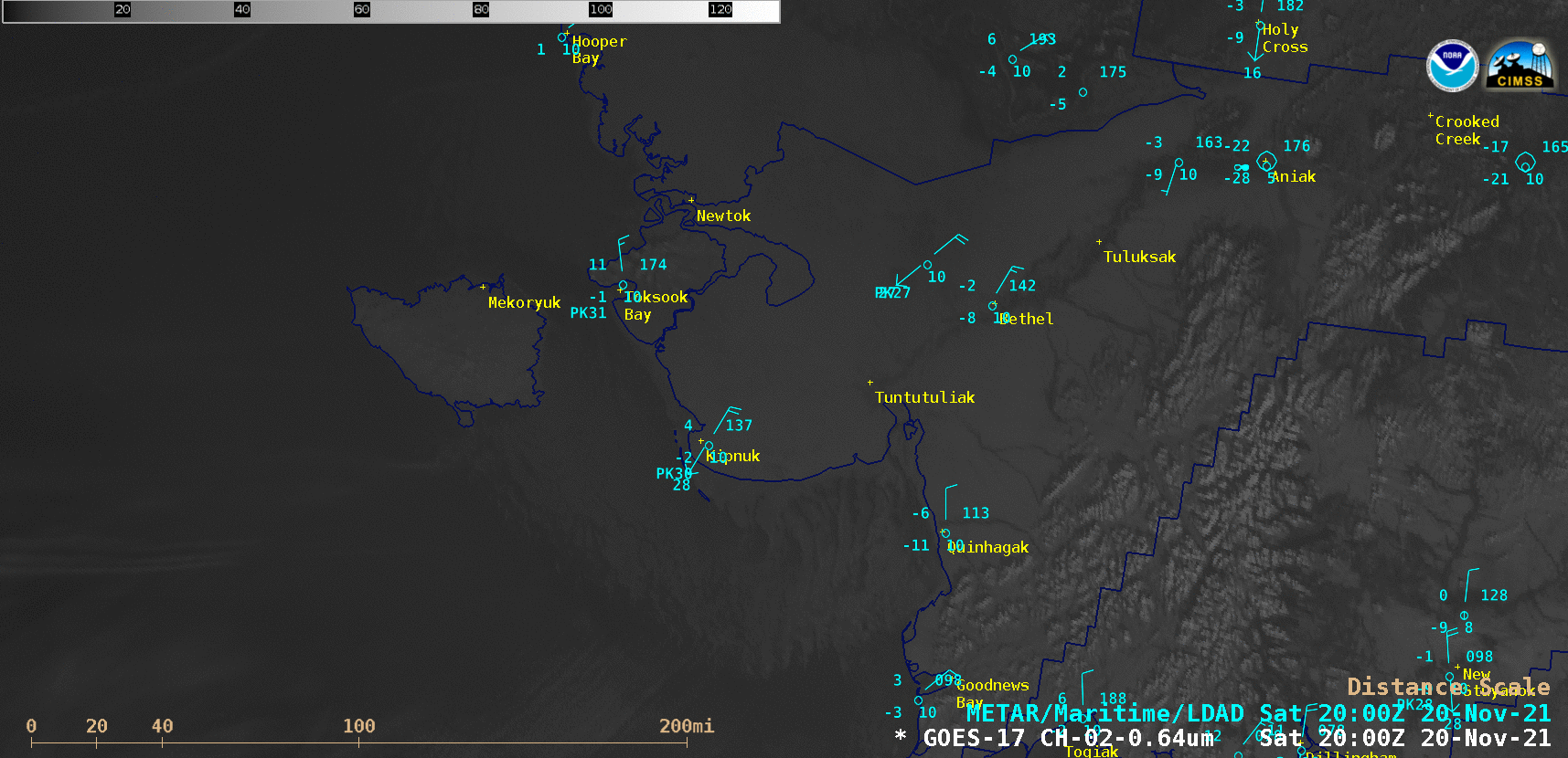
GOES-17 (GOES-West) “Red” Visible (0.64 µm) images (above) showed the motion of pack ice away from the southwest coast of Alaska on 20 November 2021. Strong offshore winds (gusting in excess of 30 knots at times) were causing the ice motion away from the coast into the Bering Sea —... Read More
GOES-17 “Red” Visible (0.64 µm) images [click to play animated GIF | MP4]
GOES-17 (GOES-West) “Red” Visible (0.64 µm) images (above) showed the motion of pack ice away from the southwest coast of Alaska on 20 November 2021. Strong offshore winds (gusting in excess of 30 knots at times) were causing the ice motion away from the coast into the Bering Sea — although some landfast ice was also evident.
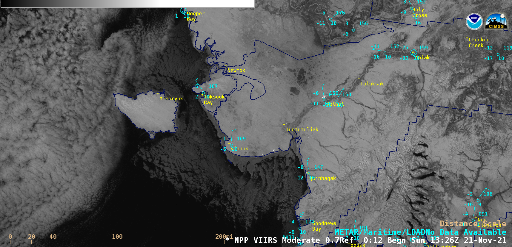
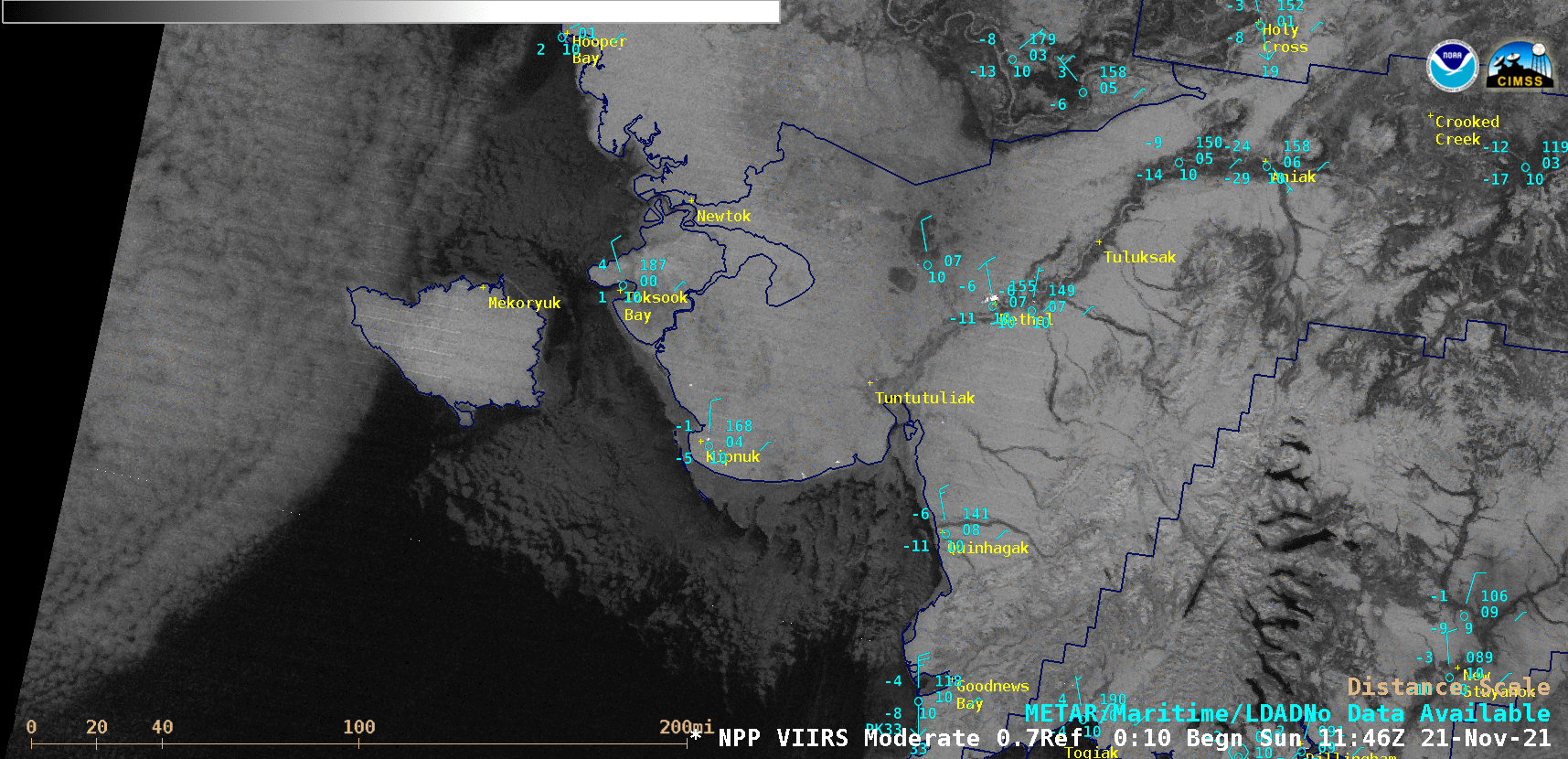
During the subsequent nighttime hours, a sequence of 3 Suomi-NPP VIIRS Day/Night Band (0.7 µm) images (below) allowed sea ice motion to be monitored during the long night, when GOES-17 Visible imagery was not available — providing that there is ample illumination from the Moon, which there was in this case (since it was in the Waning Gibbous phase, at 99% of Full).
Suomi-NPP VIIRS Day/Night Band (0.7 µm) images [click to enlarge]
This ice growth was being promoted by colder than normal Sea Surface Temperatures in that portion of the Bering Sea — along with the offshore flow of very cold air that had been in place across much of Alaska during the previous days. In fact, Interior Alaska recorded its first -40ºF/-40ºC temperatures of the winter season on this day.


