ASCAT winds versus SAR winds
From an email came this question: RADARSAT vs ASCAT winds, what are the differences between the two methods?
This comparison is not easy to make directly, as the orbits of Metop-B and Metop-C, the two satellites that carry the ASCAT instrument (now that Metop-A, which satellite also carried ASCAT, has been decomissioned), don’t sample the ocean at the same time/location as RADARSAT. The toggle above shows ASCAT winds from Metop-B (Metop-B orbits on 22 November 2021 are here, from this website) at 0631 and 1826 UTC on 22 November (from this source) in the region around Haida Gwaii (once known as the Queen Charlotte Islands). An obvious frontal passage occurred between those two times; this is also shown in the animation of surface charts (every 3 hours from 0600 through 1500 UTC shown here).
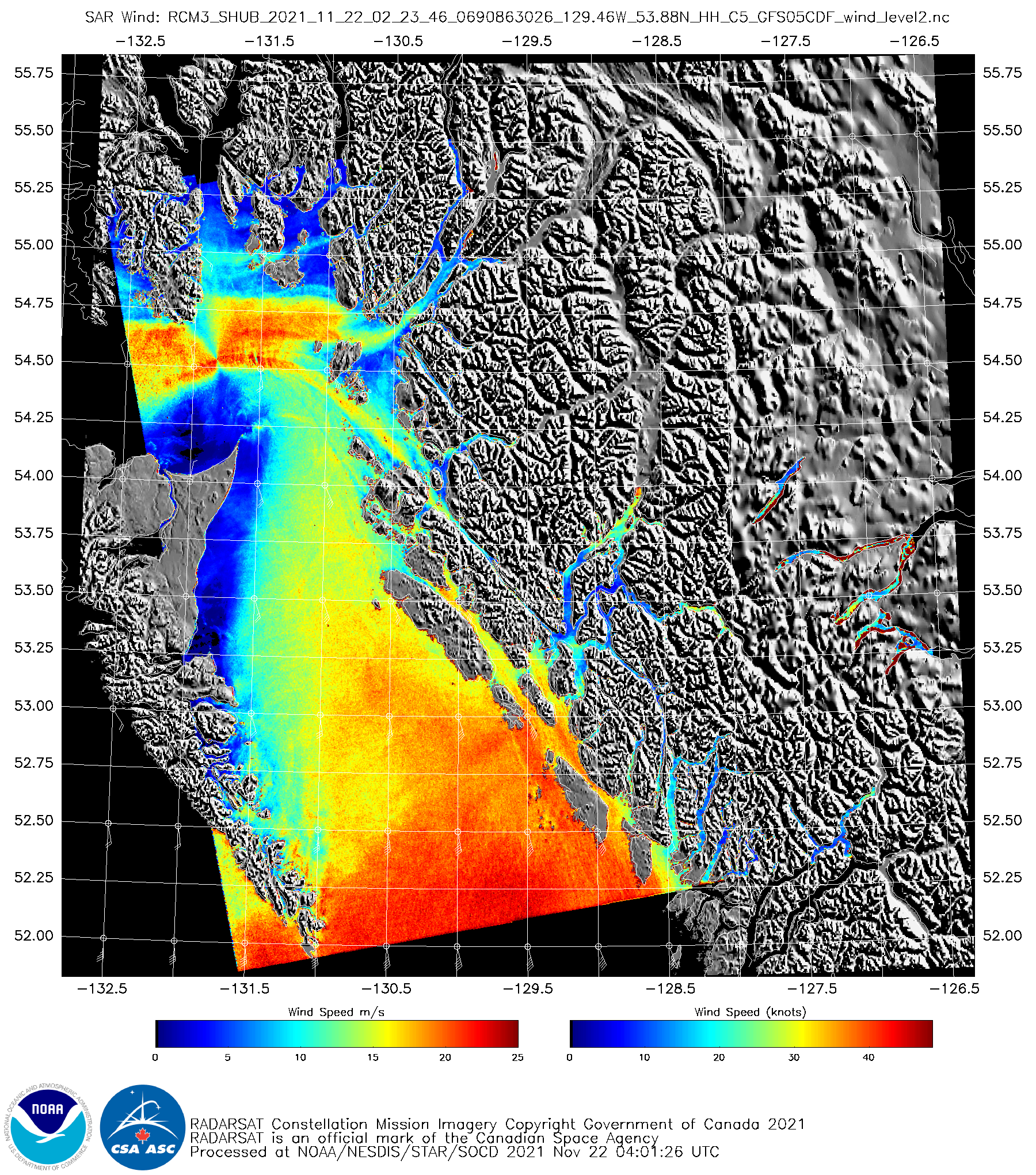
Imagery below shows SAR winds from RCM3 and RCM1 (RCM = RADARSAT Constellation Mission) at 02:23 (top) and around 15:03 (bottom) UTC on 22 November. The 15:03:52 image that follows the two images at bottom is here.
How does scatterometery measure winds? If wind speeds over the ocean (or a lake) are very light, the water surface will be smooth. Microwave energy from a side-looking radar (ASCAT and SAR are both active radars; that is, they emit a ping and listen for a response) will reflect off it, and not scatter back to the instrument. As winds increase, small ripples develop and backscatter increases. Backscattered energy is greatest if the radar look and the wind direction are aligned; also, the backscatter is greater if the wind is blowing towards (vs. away from) the satellite. This is a source of ambiguity in direction. The backscatter distribution sensed has a name: Normalized Radar Cross-Section (NRCS); many different wind speed/direction combinations can produce the same NRCS. How can you mitigate these ambiguities?
For ASCAT instruments, the ambiguity is reduced through multiple measurements of the same surface — this gives NRCS values with different aspect and incident angles. Multiple measurements are achieved via the multiple antennas that are part of the ASCAT instrument (similarly, rotating beams on instruments such as AMSR-2 give multiple observations). Multiple observations allow for an accurate estimate of wind direction given the observations.
SAR processing mitigates the ambiguities by using numerical model output that suggests the correct wind direction. A challenge is that numerical model data has a far coarser resolution than SAR data. (Model data might also include errors!) As a result, artifacts can be introduced, and a good example is shown in the 02:23 UTC image above at 54.6 N, 131.8 W. In that region, where the windspeeds have an hourglass shape, the model wind direction is unlikely to be consistent with the observations. Keep that in mind when observing SAR winds.
One other aspect of the ASCAT v. SAR wind comparison bears notice: ASCAT winds have a typical upper bound, at around 45-50 knots. At stronger wind speeds, the backscatter to the ASCAT instrument is affected by foam on the sea surface that typically accompanies such strong winds. Special SAR wind processing (as discussed here) allows for observations of much stronger winds, as shown for 2020’s Hurricane Laura, where Seninel-1 SAR observations peaked at 150 knots! These computations use cross-polarization observations from SAR. Both SAR and ASCAT use co-polarization observations. Future ASCAT missions will support cross-polarization observations.
Some of the information above came from this link (specifically, here). If there are errors in the description, they’re this blogger’s fault however.