GOES-16 (GOES-East) “Red” Visible (0.64 µm), Near-Infrared “Cirrus” (1.37 µm), Mid-level Water Vapor (6.9 µm) and “Clean” Infrared Window (10.3 µm) images (above) displayed a pattern of transverse cloud banding over parts of the Upper Midwest on 28 February 2022.  This type of transverse banding is often a signature of an enhanced potential of middle- to high-altitude turbulence — so not surprisingly, there were several pilot reports of light to moderate turbulence in the vicinity of these cloud bands.

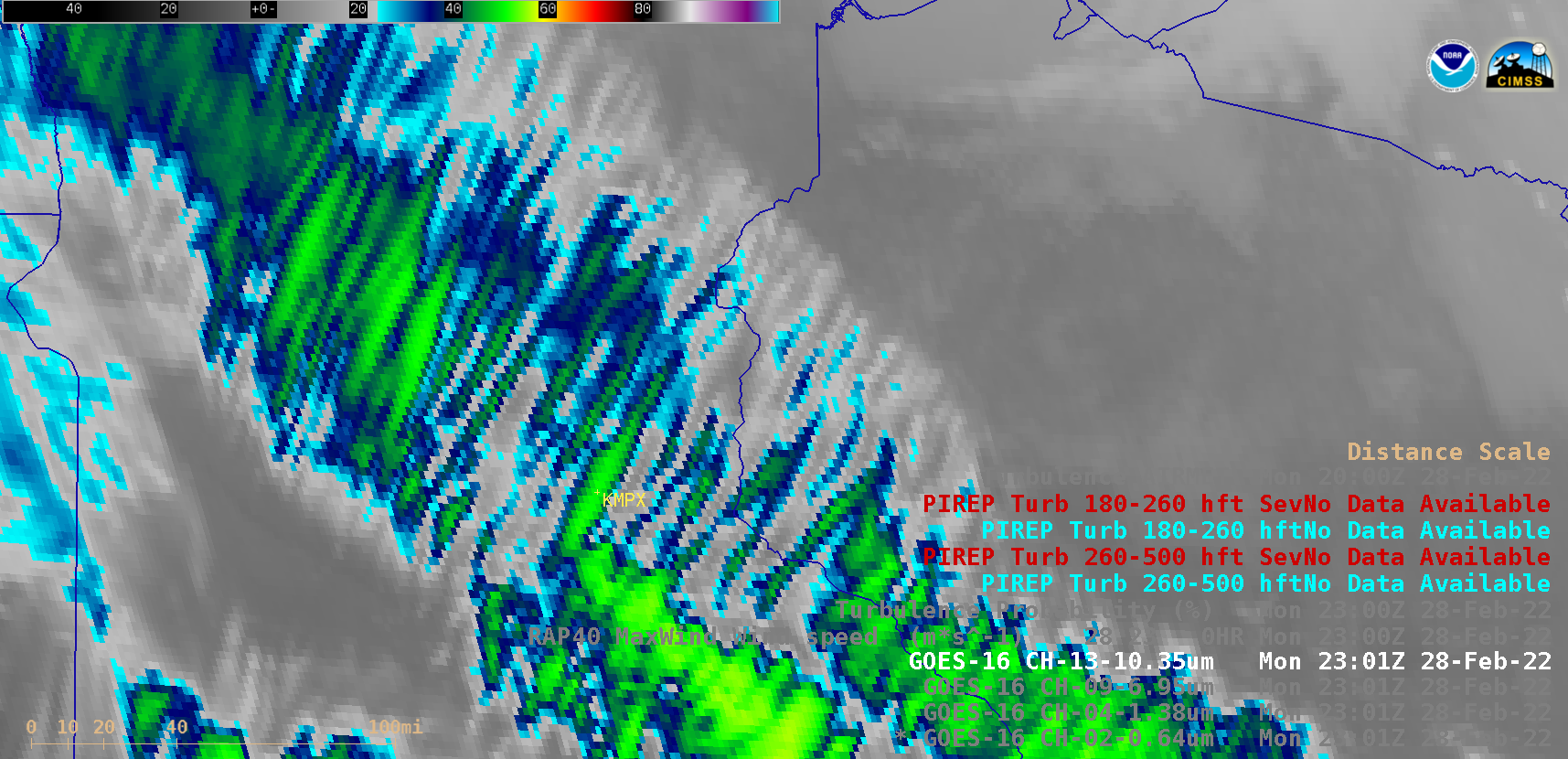
A closer view of the transverse banding over Minnesota and Wisconsin at 2301 UTC is shown below.

Hourly GOES-16 Near-Infrared “Cirrus” images with contours of RAP40 model Maximum Wind isotachs (below) indicated that this pattern of transverse banding was occurring within the left exit region of an anomalously-strong anticyclonically-curved upper tropospheric jet streak — consistent with the findings of a study by Trier and Sharman.

Such transverse banding cloud features are frequently observed around the periphery of decaying MCSs (for example, July 2020 , June 2018 and July 2016) and in the vicinity of strong upper-tropospheric jet streaks (for example, February 2020 and March 2016).

View only this post Read Less

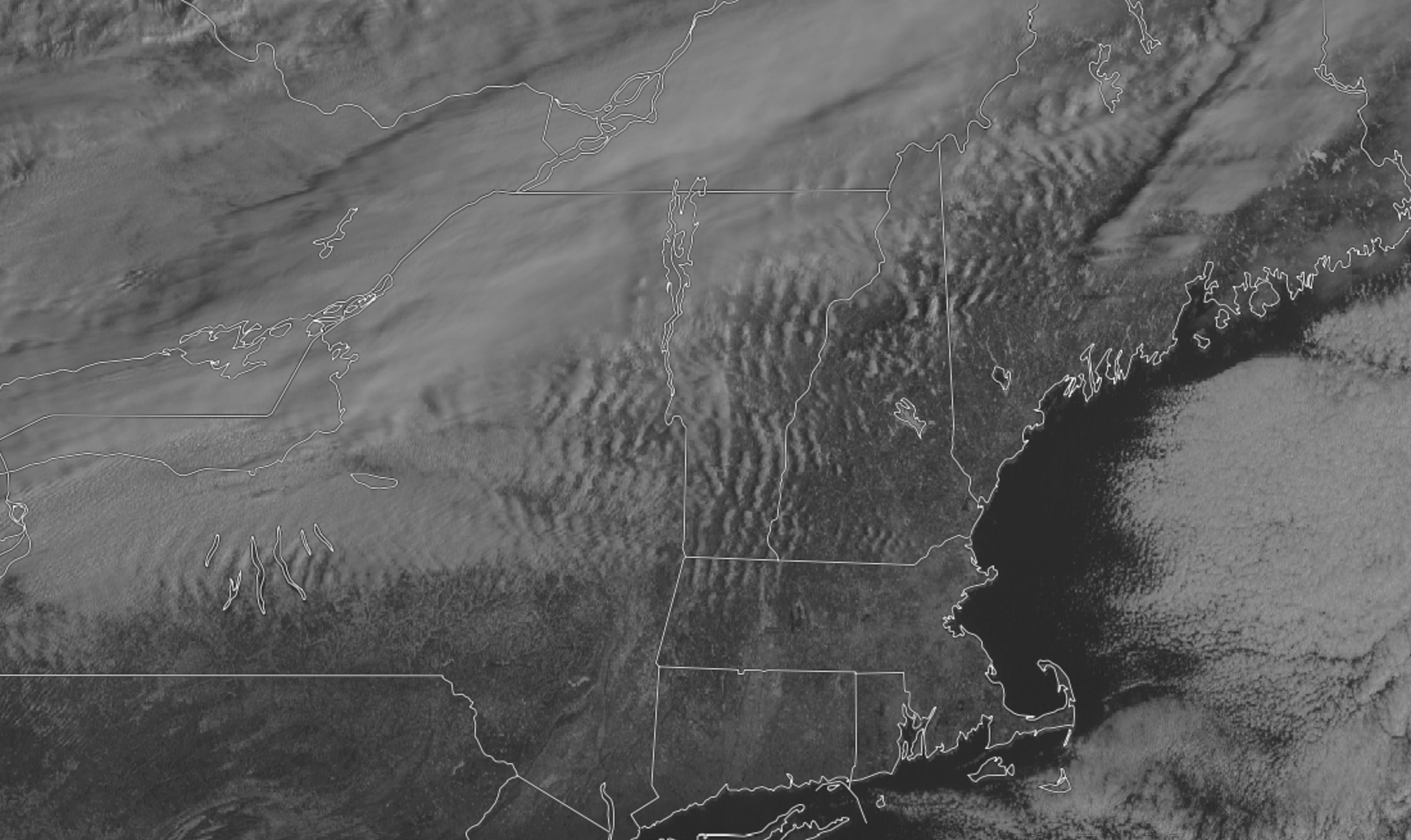
A squall warning was issued for areas of southern Quebec and Ontario as well as New York, Vermont, New Hampshire, and Maine on Sunday, February 27, 2022. The eastward moving system was surrounded by a lower deck of organized stationary wave clouds as seen in this high-resolution GOES-16 Band 2 video. The snow brought whiteout, zero visibility, conditions and wind gusts up to 40 mph.

View only this post Read Less

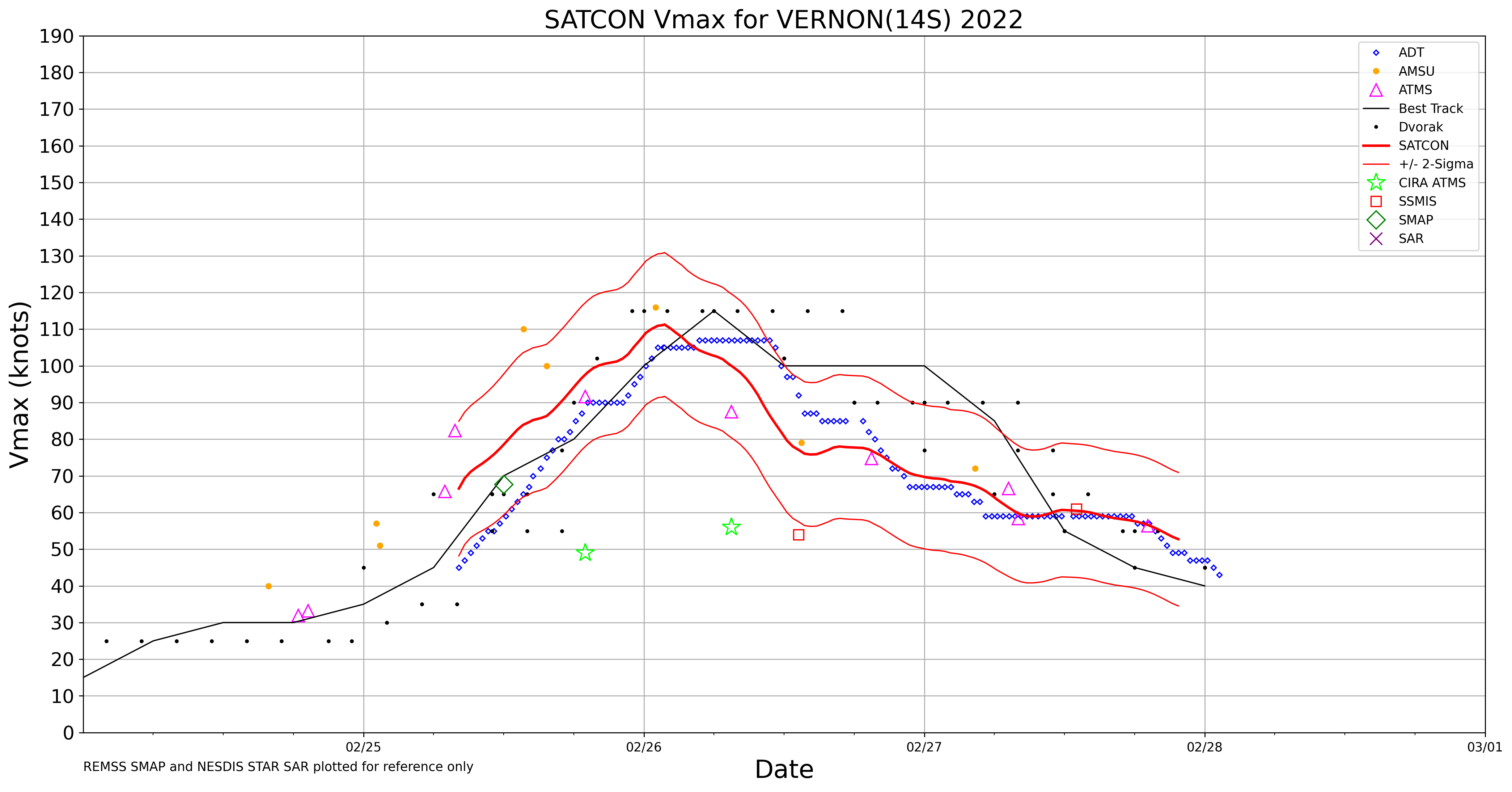
JMA Himawari-8 “Clean” Infrared Window (10.4 µm) images (above) displayed the Fujwhara effect between Cyclone Vernon (which rapidly intensified and briefly developed a small eye) and Tropical Invest 93S, as they rotated (clockwise) around each other in the South Indian Ocean — west of Cocos Island, station identifier YPCC — during the 25 February – 27 February 2022 period. Invest 93S was eventually absorbed by Vernon (which decreased in intensity during the absorption  process).

Himawari-8 “Red” Visible (0.64 µm) images (below) showed Vernon when it had reached a peak intensity of Category 3 (ADT | SATCON) — however, the eye remained cloud-filled during that time.

View only this post Read Less

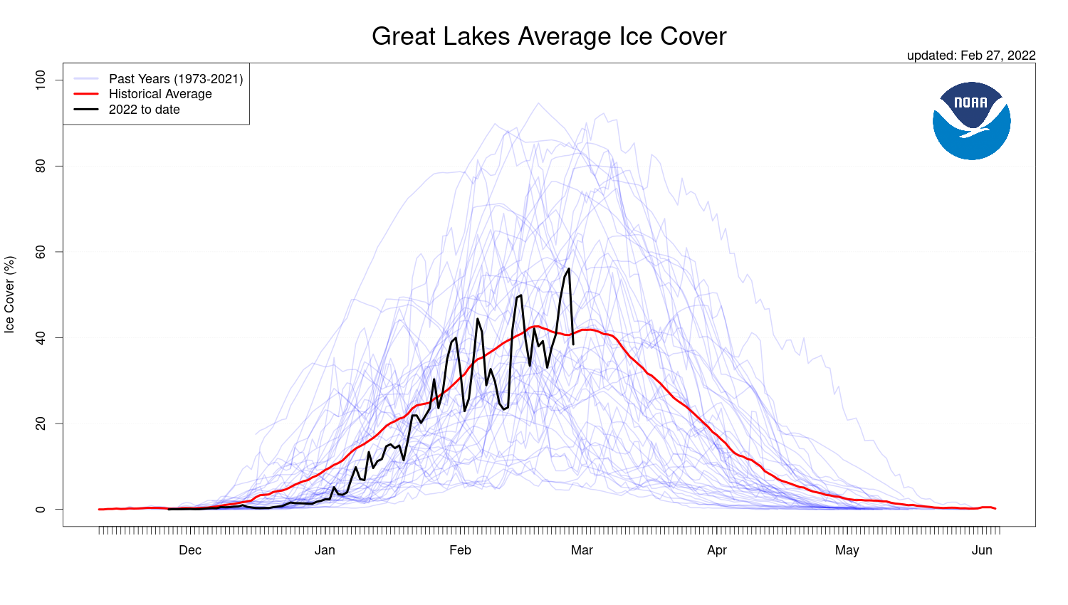
A colder-than-normal February over the western Great Lakes (through the 27th, Duluth is 10^o F below normal; Marquette is 5^o F below normal; Green Day is 2^o F below normal; Cleveland is 1^o F below normal) has fostered a growth in ice cover over the Lakes (This figure, from here, for example). How can satellites detect that ice, especially for a region where winter-time cloudiness is notorious? In general, there are two different ways to detect ice: Visible/Infrared imagery and Microwave imagery. The toggle above shows Advanced Technology Microwave Sounder (ATMS) ice detection (using MiRS algorithms and data from Suomi-NPP (1807 UTC) and NOAA-20 (1859 UTC)) over the Great Lakes on 25 February 2022. (These data come from the Direct Broadcast antenna at CIMSS, and are processed using CSPP to produce AWIPS-ready tiles that are available via an LDM feed). A big challenge with this field is the very large ATMS footprint. Note that these sea-ice concentration values are quantitative: values change based on how much ice is within the footprint but are also dependent on view angle.

VIIRS data (as shown at the VIIRS Today website, for example) can also be used to infer regions of ice in a qualitative sense, as shown below. The true color imagery shows possible ice features over the lakes. It’s a challenge, however, to use a single VIIRS image to distinguish (mostly) stationary ice from (usually) moving clouds. Multispectral VIIRS imagery means (via the use below of the 2.25 µm M11 band) ice features are cyan colored and can be qualitatively distinguished from clouds. Consider, for example, the color difference in the False Color image between the clouds over eastern Lake Superior (white in both True- and False-Color) and near-shore ice over southern and eastern Lake Superior (white in the True-Color and cyan in the False-Color). There are also VIIRS-based Ice Concentration products that can be computed in clear skies.

---

For cloudy regions, Advanced Baseline Imagery can be used to create estimates of Ice Surface Temperature and Ice Concentration. Quantitative estimates such as these give more information than the qualitative estimates shown above. These estimates at present are only created hourly; in partly-cloudy regions, that cadence is sufficient to give lake-wide quantitative estimates of ice coverage and temperature. CONUS imagery — with a 5-minute time cadence — and mesoscale sectors — with 1-minute cadences — can be used to monitor (in a qualitative sense) how ice is moving (as shown link, for example). High temporal-resolution imagery is important because ice sheets can change rapidly under strong winds, as shown in this tweet. At high latitudes, there are also ways of monitoring ice motion via polar orbiters (link).

---

A much higher-resolution method of viewing ice (again, in a qualitative, not quantitative sense) in regions of both clear and cloudy skies, day or night, is through the use of Synthetic Aperture Radar (SAR). Data are available for each Great Lake at this link. Imagery for each Lake over the past days is available there, albeit infrequently (usually around 0000 and 1200 UTC only) and over small domains. This qualitative imagery, however, is very high-resolution and gives very impressive details. Imagery over Lake Erie is shown below.

---

VIIRS and ABI give both qualitative (false-color, visible imagery) and quantitative (ice concentration and ice temperature) depictions of ice over the lakes — or over coastal waters around Alaska. Microwave data also gives quantitative estimates (ice concentrations with large microwave footprints) and qualitative estimates (SAR data). Use all products to create a clear picture of ice coverage.

View only this post Read Less