This blog post contains Suomi-NPP VIIRS imagery that was derived (using CSPP) from data downloaded at the Direct Broadcast site at CIMSS. That blog post suggests the need of a brightness temperature difference field from the I04 and I05 data that can be found in this (https://ftp.ssec.wisc.edu/pub/eosdb/npp/viirs/2022_03_03_062_0632/sdr) direct broadcast directory (direct link, available for about 6 days). The Sensor Data Record directory includes I04 and I05 hdf5 granules that McIDAS-V can read: SVI04_npp_d20220303_t0641201_e0642443_b53613_c20220303071038095682_cspp_dev.h5 and SVI05_npp_d20220303_t0641201_e0642443_b53613_c20220303071039605225_cspp_dev.h5 ; determining exactly which granule you want — there are 10 different granules in this particular directory — is partly trial and error and partly viewing the orbit path (here) and choosing wisely. Save those files into a directory; also save the ‘GITCO’ files (that is: GITCO_npp_d20220303_t0641201_e0642443_b53613_c20220303070838040363_cspp_dev.h5) that contain georeferencing for the Imager (‘I’) bands (similarly, GMTCO files contain georeferencing for the Moderate-resolution ‘M’ bands).

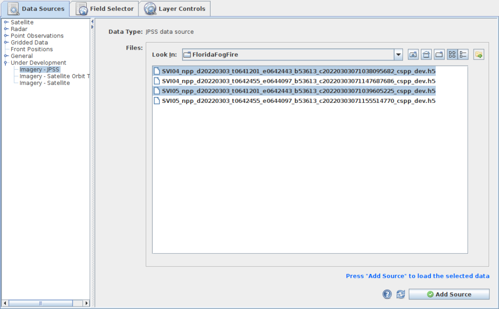
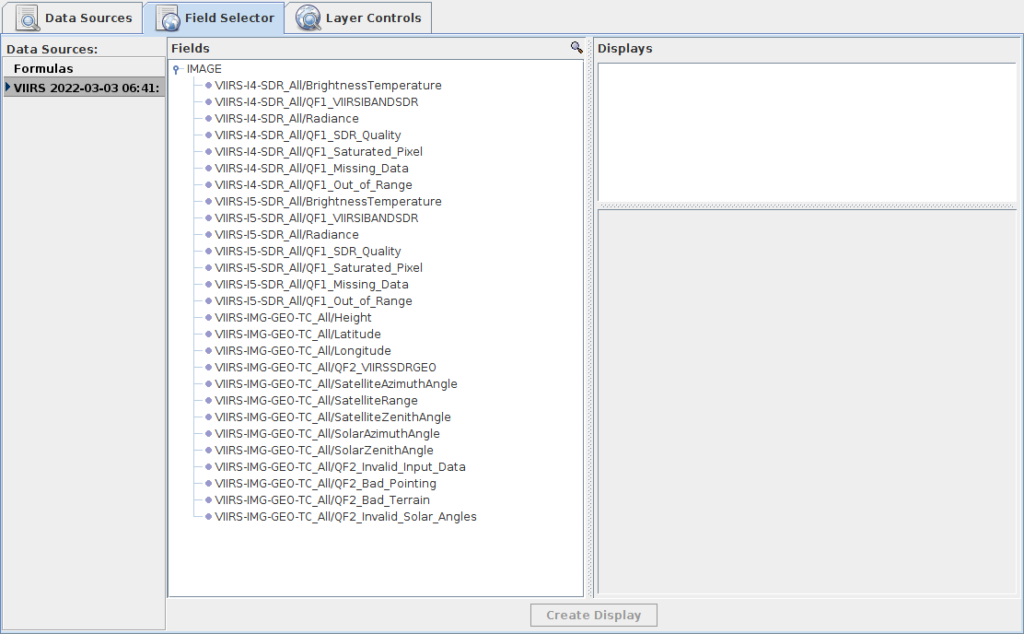
After starting up McIDAS-V, you want to load the data. Note above that I’ve clicked on JPSS Imagery, and navigated to the directory containing the downloaded data (that directory also includes the GITCO files for those granules, but you don’t see them here). I’ve chosen both I04 and I05 data files from one granule, observed from 06:41:20.1 to 06:42:44.3. Click on ‘Add Source’ in the lower right corner of the window. If you then expand ‘IMAGE’ under ‘Fields’, you’ll see both I04 and I05 Brightness Temperatures.

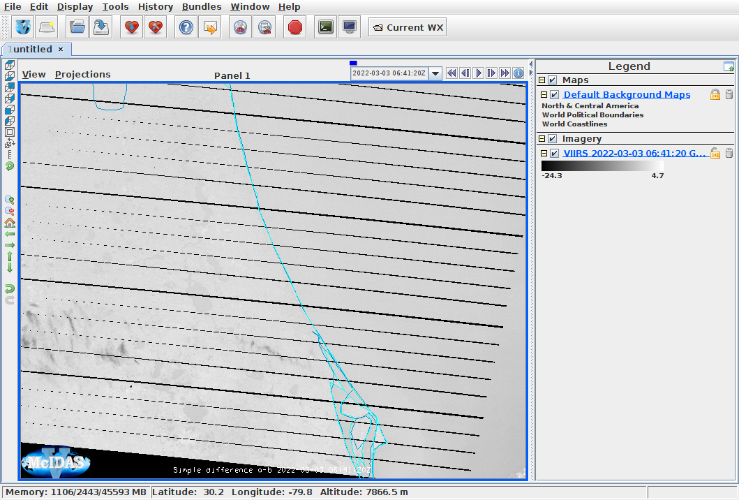
Next, under the ‘Data Sources:’ tab, click on ‘Formulas’. You will see a ‘Miscellaneous’ tab, and under that tab, a ‘Simple Difference a-b’ choice. Choose that and click ‘Create Display’ — this will pop up a window in which you can choose the a (in this case, I05 Brightness Temperature) and b (for this case, I04 Brightness Temperature). Subsect the portion of the granule that you want to display using shift-left click and drag — and — after clicking ‘create image’ — you end up with the image below (zoomed in).

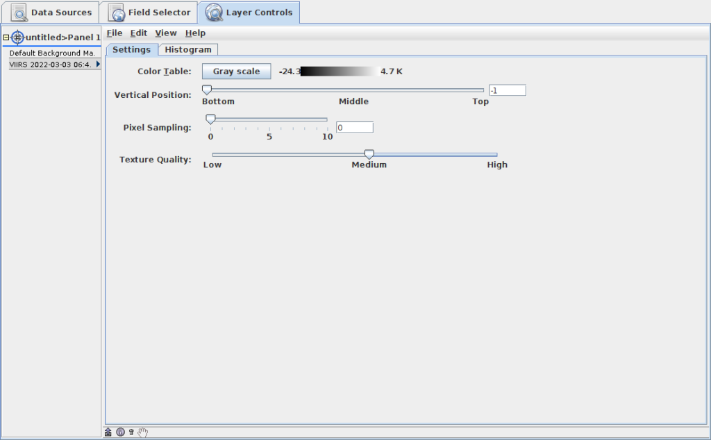
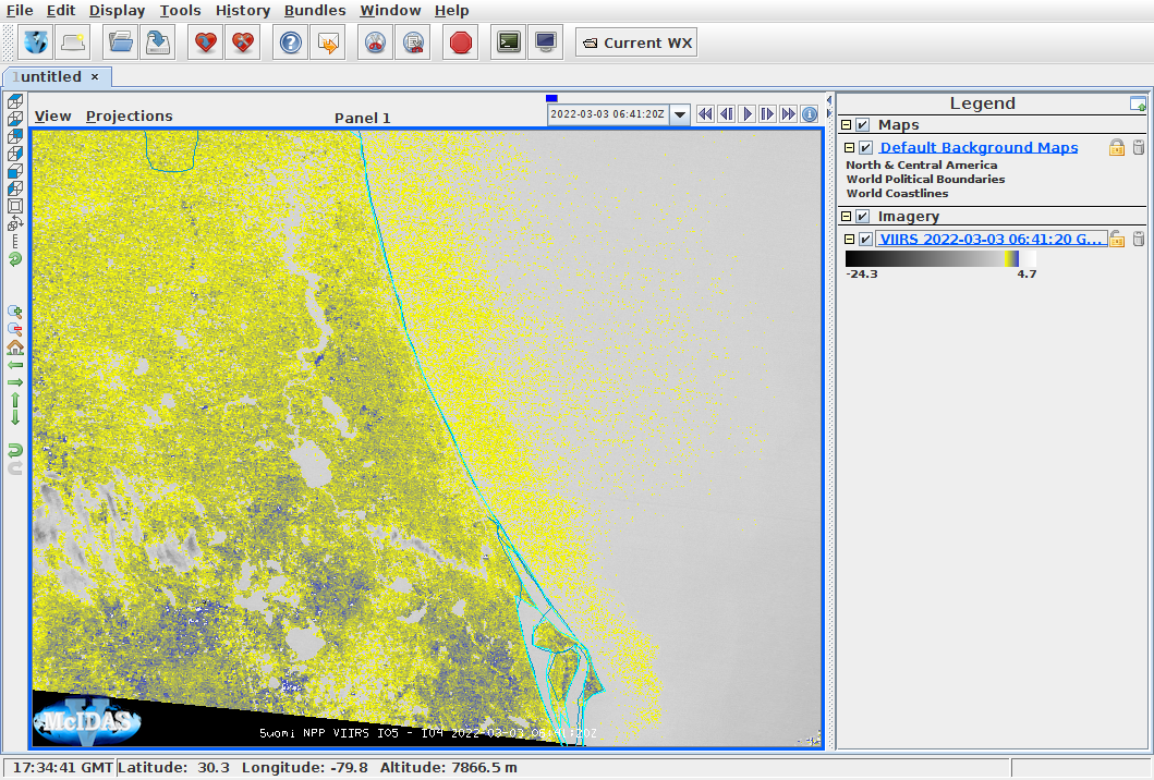
There is some fine-tuning yet to do. Under the ‘Legend’ in the image above, right-click on ‘VIIRS 2022-03-03…’ to bring up the Control Window shown below. Slide the ‘Texture Quality’ from ‘Medium’ to ‘High’ (if you have a large image — much larger than this one! — that will test your machine’s RAM!)

Similarly, if you right-click (again!) under ‘Legend’ and ‘VIIRS 2022-03-03…’ to ‘Edit->Properties’, you can change the Layer Label to include more information, which I did, as shown in the image below. Finally, I edited the color table to highlight positive values (that is, where I05 – I04 Brightness Temperature Difference is between 0 and 2^o C) that might show where stratiform clouds are present. That result is shown below. Yellow in the enhancement shows no difference between the fields, blue is a brightness temperature difference of 2^o C. Are you obtaining a good signal of fog in the region of the very dense fog over southern Volusia County? I’d only ask what a ‘good signal’ is!

Imagery in this post was created using v1.8 of McIDAS-V (downloadable here). You can find further documentation on this here.

View only this post Read Less

GOES-16 (GOES-East) Shortwave Infrared (3.9 µm), Fire Temperature RGB. Fire Power, Fire Temperature and Fire Area products (above) displayed signatures of widespread prescribed and/or agriculture fires across parts of the Southern Plans and Lower Mississippi Valley on 03 March 2022. The Fire Power, Fire Temperature and Fire Area derived products are components of the GOES Fire Detection and Characterization Algorithm FDCA; Fire Temperature values were as high as 2300 K, with Fire Power values reaching 220 MW for some of the hottest fires.

Even though the majority of these fires were relatively brief and rather small in areal coverage, many produced notable smoke plumes — which were highlighted by GOES-16 True Color RGB images created using Geo2Grid (below). This smoke reduced the surface visibility to 7-9 miles at a few locations, but one site in southern Missouri reported a visibility as low as 3/4 mile.

View only this post Read Less

A combination of fog and smoke reduced visibilities along I-95 S in southern Volusia County Florida. A series of fatal crashes (news report; this tweet suggests the accident was near Florida State Route 442; second tweet). News report suggest the smoke that helped seed the dense fog resulted from controlled burns. The Band 7 imagery (3.9 µm) above, does not show strong evidence of burns (the Fire Detection and Characterization Algorithm — FDCA — similarly showed no information in Volusia County), nor of the fire that occurred at the crash scene as vehicles burned. The first crashes occurred around 0630 UTC.

The Nighttime microphysics RGB is often used to highlight regions of fog. On this day, however, no obvious signal of fog (fog typically appears as a color between cyan and yellow, as noted here) is apparent.

The Night Fog brightness temperature difference (the ‘green’ component of the RGB above) also can be used to detect fog. GOES-R IFR Probability fields use satellite data (and model data) to outline regions of fog. The toggle below includes the night time microphysics RGB, the night fog brightness temperature difference, and the IFR Probability fields at 0631 UTC, near the time of the crash. Satellite data provided little detection for this very thin combination of smoke and fog. For this case, it would be better to rely on things like webcams.

---

There was a very timely Suomi-NPP overpass as shown below. The timestamp is at 0632 UTC, which is when the satellite first was broadcasting data to the Direct Broadcast antenna at CIMSS; the satellite was viewing central Florida around 0642 UTC, based on this orbit calculation (from this site). The slider does suggest a small temperature difference as might be caused by fog over southern Volusia County. (Click here to see a toggle — and here to see a very fast toggle).

A brightness temperature difference field between I05 and I04 on this date was created using McIDAS-V in this blog post.

———————————————————————————————————-

A similar incident of fog — possibly enhanced by smoke — causing a multi-vehicle accident occurred in Osceola County (not far to the south of Volusia County) Florida on 13 March 2007. In that case, higher-resolution MODIS imagery was a bit more helpful in helping to highlight an area of nocturnal fog formation.

View only this post Read Less

Turbulence probability is an aviation tool created (using machine learning techniques) at CIMSS to diagnose the likelihood of Moderate Or Greater (MOG) turbulence at least once during a 10-minute period. The image above shows the 1455 UTC MOG Turbulence Probability along with pilot reports (PIREPS) of turbulence, taken from this website. Turbulence Probability fields are also in AWIPS, and the 1500 UTC image is shown below.

There are frequently features in the water vapor imagery (or in visible, or near-infrared, imagery during the day) that have a known association with turbulence. The turbulence probability field is toggled below with the 6.19 µm upper-level water vapor infrared imagery, and beneath that with the 1.38 µm “cirrus band” near-infrared imagery. Striated features that are apparent in, for example, this event from 28 February, are not obvious.

MOG Turbulence Probability also includes information from the GFS: temperature, height, and winds from 850 mb to 50 mb! (Such GFS fields are especially important when using GOES-17 data during times when the Loop Heat Pipe malfunctions leads to data loss over the Pacific.) The toggles below show the relationship between the Turbulence Probability and upper-tropospheric stability (as diagnosed by the 400-300 mb lapse rate), and the also the pressure on the 1.5 PVU surface. Turbulence is occurring just Equatorward of a slope in the tropopause, in a region of weak stability.

GOES Data can also be used to diagnose wind speeds in the upper-troposphere. Peak winds in the 350-450 mb layer, shown in a toggle below with the MOG Turbulence Probability, are 100-120 knots from southeastern North Dakota into northwestern Wisconsin.

How did this potential for turbulence (and strong winds) affect air traffic? Consider the path of one late-morning flight, Delta Flight 867 from Minneapolis to Seattle. Its path is shown below for February 28th, and for March 2nd, courtesy of FlightAware. The 2 March flight was diverted south to avoid the strong winds and potential for turbulence.

---

You might ask: Why are the upper-tropospheric lapse rates shown? The reason is because they align the use of the 6.19 µm imagery. The (new and improved!!) CIMSS Weighting Function page shows that at 1200 UTC, much of the signal in the upper-level water vapor imagery (in brown in the plot below) around Minneapolis was coming from the 300-400 mb layer. A plot using GFS data at 45^o N, 95^o W, shows a similar distribution.

---

AWIPS imagery in this blog post was created using the NOAA/NESDIS TOWR-S AWIPS Cloud Instance.

View only this post Read Less