This website works best with a newer web browser such as Chrome, Firefox, Safari or Microsoft
Edge. Internet Explorer is not supported by this website.
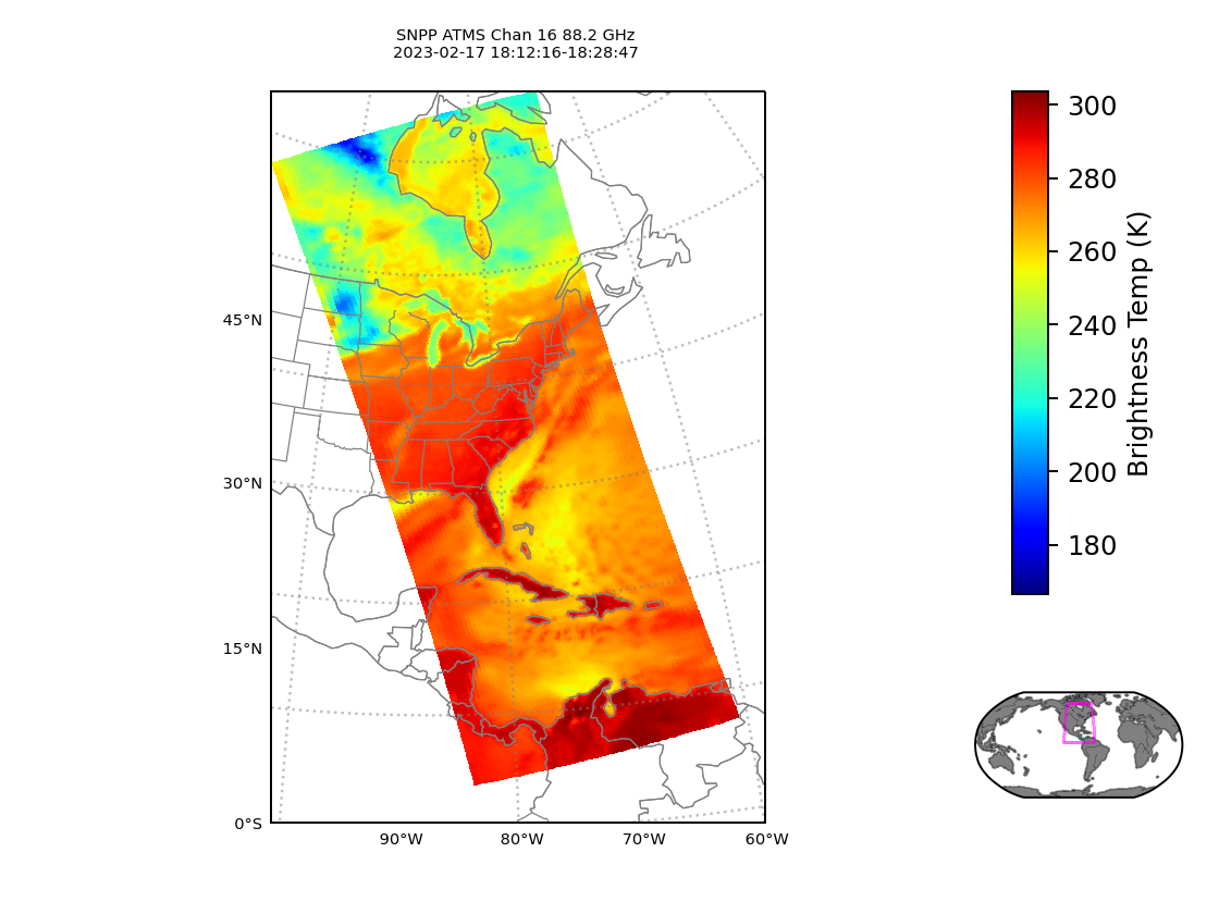
New software now in use at CIMSS combines JPSS Raw Data Records (RDRs) from Suomi-NPP or from NOAA-20, created at different direct broadcast antenna sites (for example, at CIMSS (data link for NOAA-20; data link for Suomi NPP) — and at AOML in Miami), into a single RDR that includes data that can span roughly 1/4 of a JPSS... Read More
New software now in use at CIMSS combines JPSS Raw Data Records (RDRs) from Suomi-NPP or from NOAA-20, created at different direct broadcast antenna sites (for example, at CIMSS (data link for NOAA-20; data link for Suomi NPP) — and at AOML in Miami), into a single RDR that includes data that can span roughly 1/4 of a JPSS orbit. Polar2Grid software then produces exceptional (and exceptionally long!) imagery, such as the True Color image from Suomi NPP shown below, from 1811 UTC on 17 February (also available at the CIMSS Direct Broadcast site here, or at the VIIRS Image Viewer). The view below extends from northern Canada to the Equator and includes the Pacific Ocean south of Mexico and also Lake Maracaibo in Venezuela. VIIRS single-channel and True- and False-Color imagery are produced over the larger domain; ATMS imagery is also produced over a larger domain (here’s an example 88.2 GHz image, for example, from 1811 UTC on 17 February) and extended Advanced Clear-Sky Processor for Ocean (ACSPO) SST fields are also produced that include data over the Pacific ocean southwest of Mexico, as in this example from NOAA-20 from 1918 UTC on 16 February.
Suomi NPP VIIRS True-Color imagery, 1811 UTC on 17 February 2023 (Click to enlarge greatly)
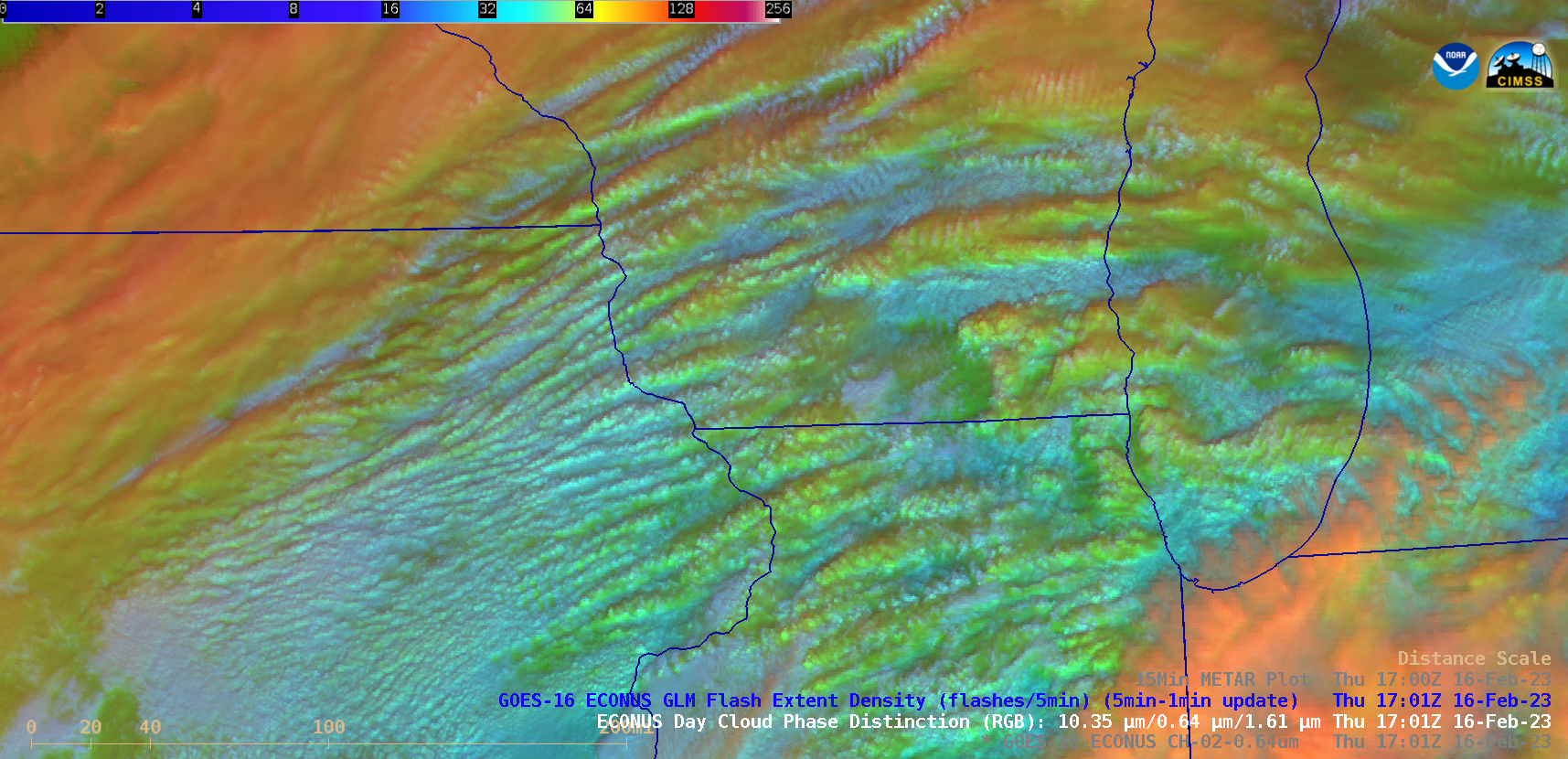
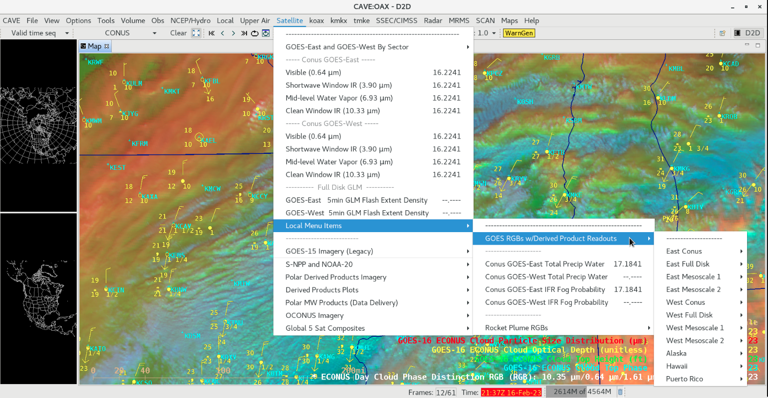
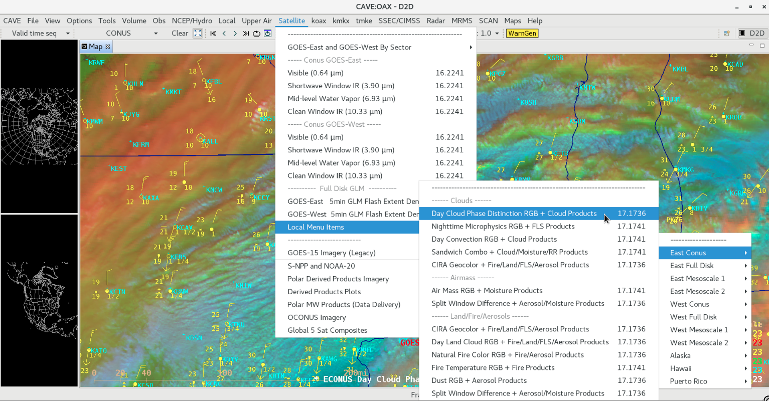
GOES-16 (GOES-East) “Red” Visible (0.64 µm) and Day Cloud Phase Distinction RGB images (above) showed widespread elevated convective banding that was helping to enhance snowfall rates — with some locations reporting 1.5 to 2.0 inches per hour — across parts of Minnesota, Wisconsin, Lower Michigan, Iowa and Illinois on 16 February 2023. There was no GLM indication... Read More
GOES-16 “Red” Visible (0.64 µm) and Day Cloud Phase Distinction RGB images, with and without plots of 15-minute METAR surface reports [click to play animated GIF | MP4]
GOES-16 (GOES-East) “Red” Visible (0.64 µm) and Day Cloud Phase Distinction RGB images (above) showed widespread elevated convective banding that was helping to enhance snowfall rates — with some locations reporting 1.5 to 2.0 inches per hour — across parts of Minnesota, Wisconsin, Lower Michigan, Iowa and Illinois on 16 February 2023. There was no GLM indication of lightning activity associated with any of these convective bands.
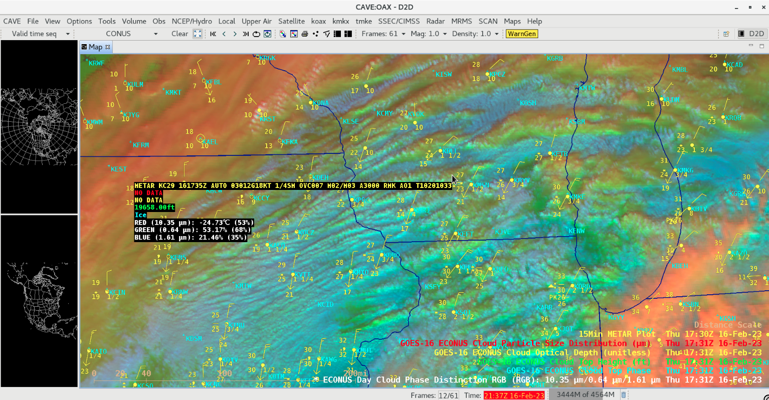
On the Day Cloud Phase Distinction RGB images, shades of yellow to green suggested that cloud tops along many of the convective bands were either glaciated or were mixed phase (composed of ice crystals and supercooled water droplets). The ability to load select GOES RGB images combined with various GOES Level 2 Derived Products (using Satellite > Local Menu Items > Satellite Sector) provides the ability to use AWIPS cursor sampling to determine specific quantitative properties associated with the various RGB shades — for example, the GOES-16 Day Cloud Phase Distinction RGB image at 1731 UTC (below) includes cursor sampling of the individual RGB components in addition to the associated Cloud Top Phase (Ice) and Cloud Top Height (19,658 feet) derived products at that cursor location, which was along a convective band that was enhancing snowfall rates and reducing the surface visibility to 1/4 mile at Middleton (KC29) just west of Madison, Wisconsin (KMSN). The GOES-16 “Clean” Infrared Window (10.3 µm) cloud-top infrared brightness temperature — the Red component of the RGB image — at that particular cursor location was -24.73ºC.
GOES-16 Day Cloud Phase Distinction RGB image at 1731 UTC, with cursor sampling of the RGB components along with Cloud Top Phase and Cloud Top Height [click to enlarge]
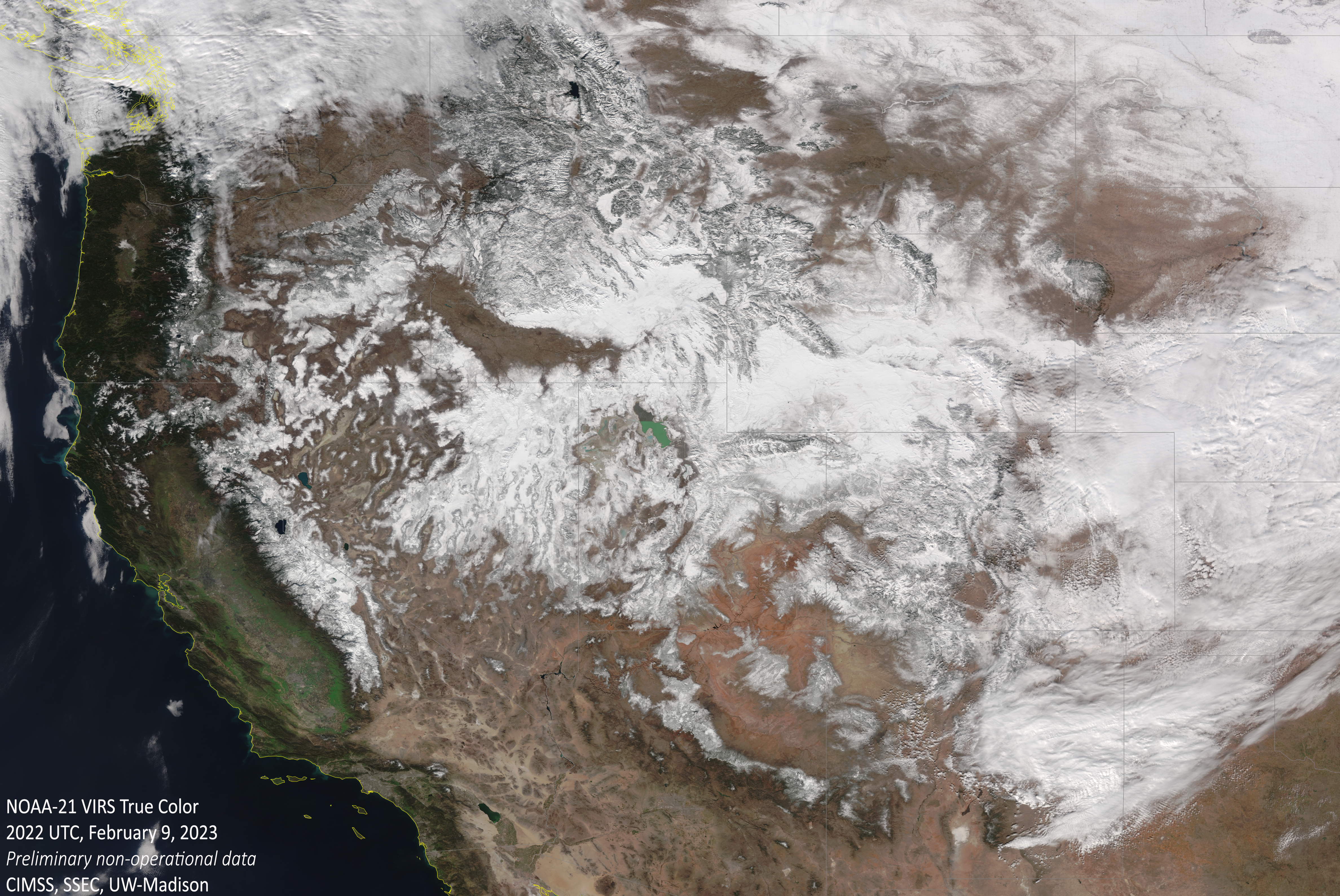
NOAA’s newest satellite, NOAA-21, has started sending data to Earth with each overpass. The satellite launched 3 months ago as JPSS-2, and was renamed NOAA-21 once in orbit. NOAA-21 joins the Suomi-NPP and NOAA-20 satellites in polar orbit around Earth. CIMSS acquires NOAA-21 views of North America via Direct Broadcast... Read More
NOAA’s newest satellite, NOAA-21, has started sending data to Earth with each overpass. The satellite launched 3 months ago as JPSS-2, and was renamed NOAA-21 once in orbit. NOAA-21 joins the Suomi-NPP and NOAA-20 satellites in polar orbit around Earth.
True Color image of the western U.S. acquired by the Visible and Infrared Imaging Radiometer Suite (VIIRS) on February 9th, 2023.
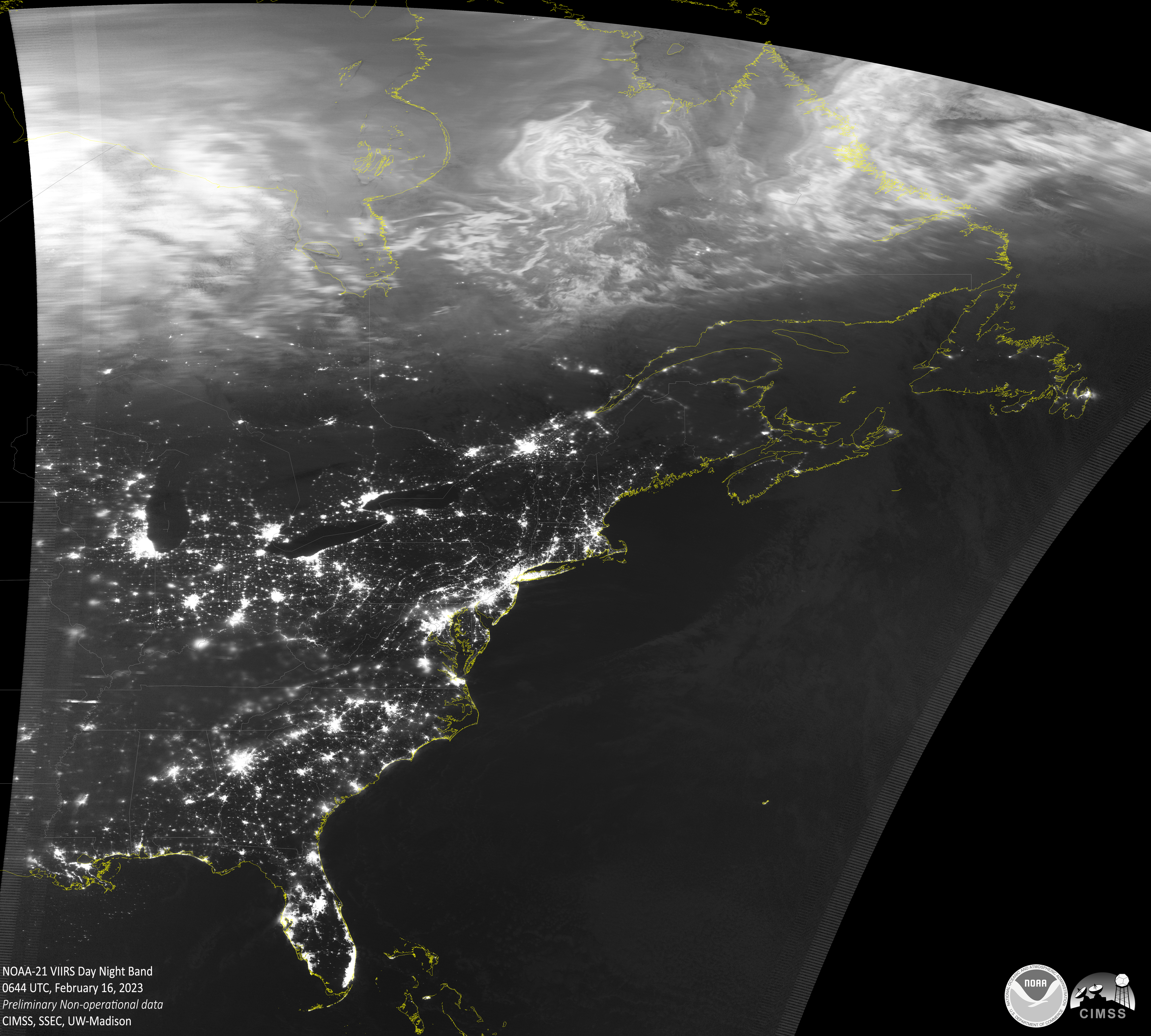
NOAA-21 Day Night Band Aurora Borealis image from February 16th, 2023
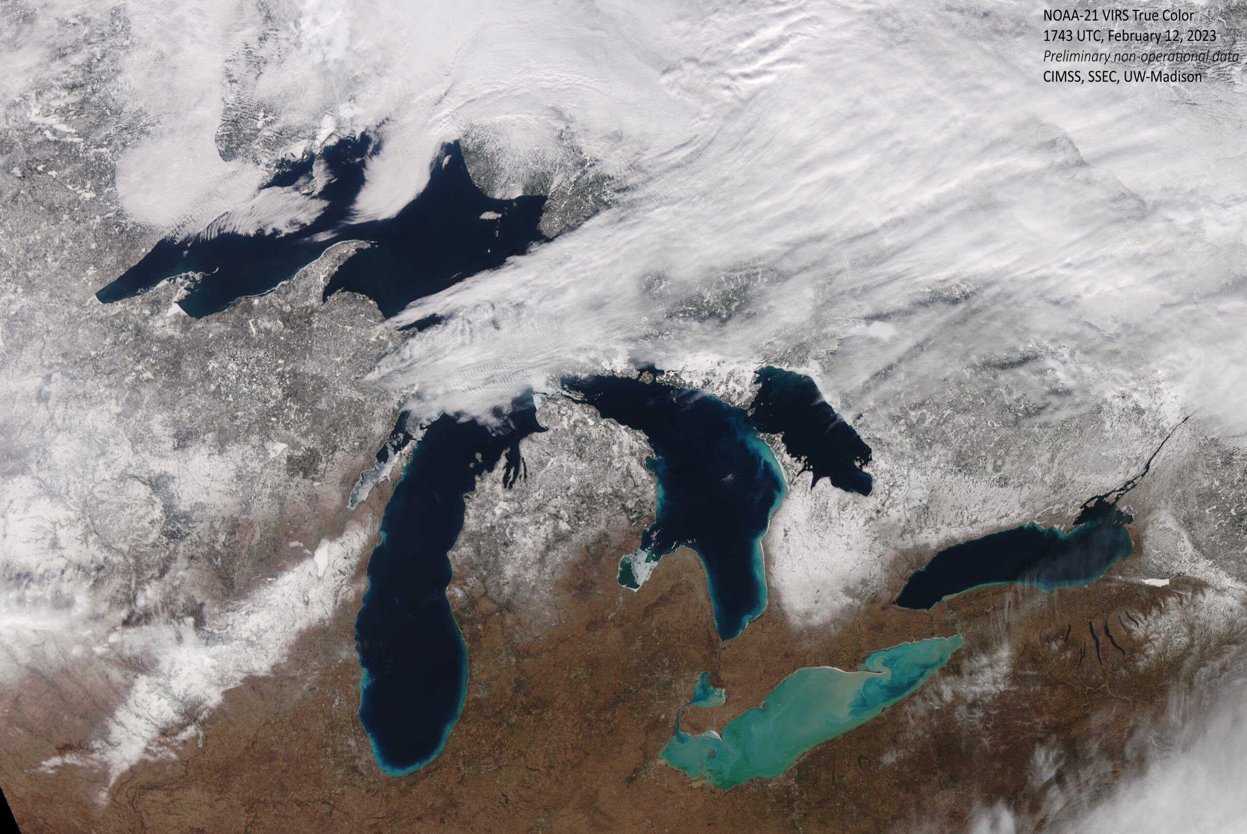
NOAA-21 VIIRS True Color Great Lakes scene from February 12th, 2023
CIMSS acquires NOAA-21 views of North America via Direct Broadcast from the satellite to a receiver on our roof when NOAA-21 flies overhead. NOAA is receiving global NOAA-21 data and shared the following images.
NOAA-21 M15 Band Brightness Temperature global composite from February 9-10, 2023
NOAA-21 VIIRS Day Night Band global composite from February 9–10, 2023
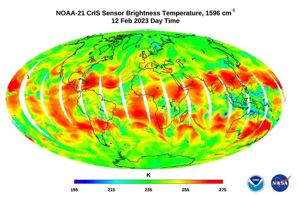
NOAA-21 CrIS global composite from February 12, 2023
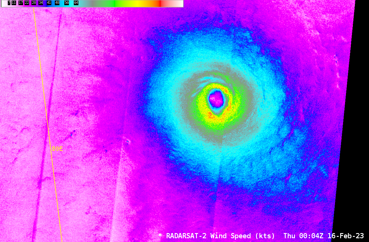
RADARSAT-2 and RCM-1 had two closely-spaced overpasses over Cyclone Freddy in the Indian Ocean early on 16 February 2023, as shown above. Eyewall speeds exceed 130 knots in the RCM-1 data! (Imagery and data are available here). The quadrant analyses for RCM-1 and for RADARSAT-2 show hurricane-force winds extending out... Read More
RADARSAT and RCM1 SAR Winds over Cyclone Freddy, 0004 and 0012 UTC on 16 February 2023 (Click to enlarge)
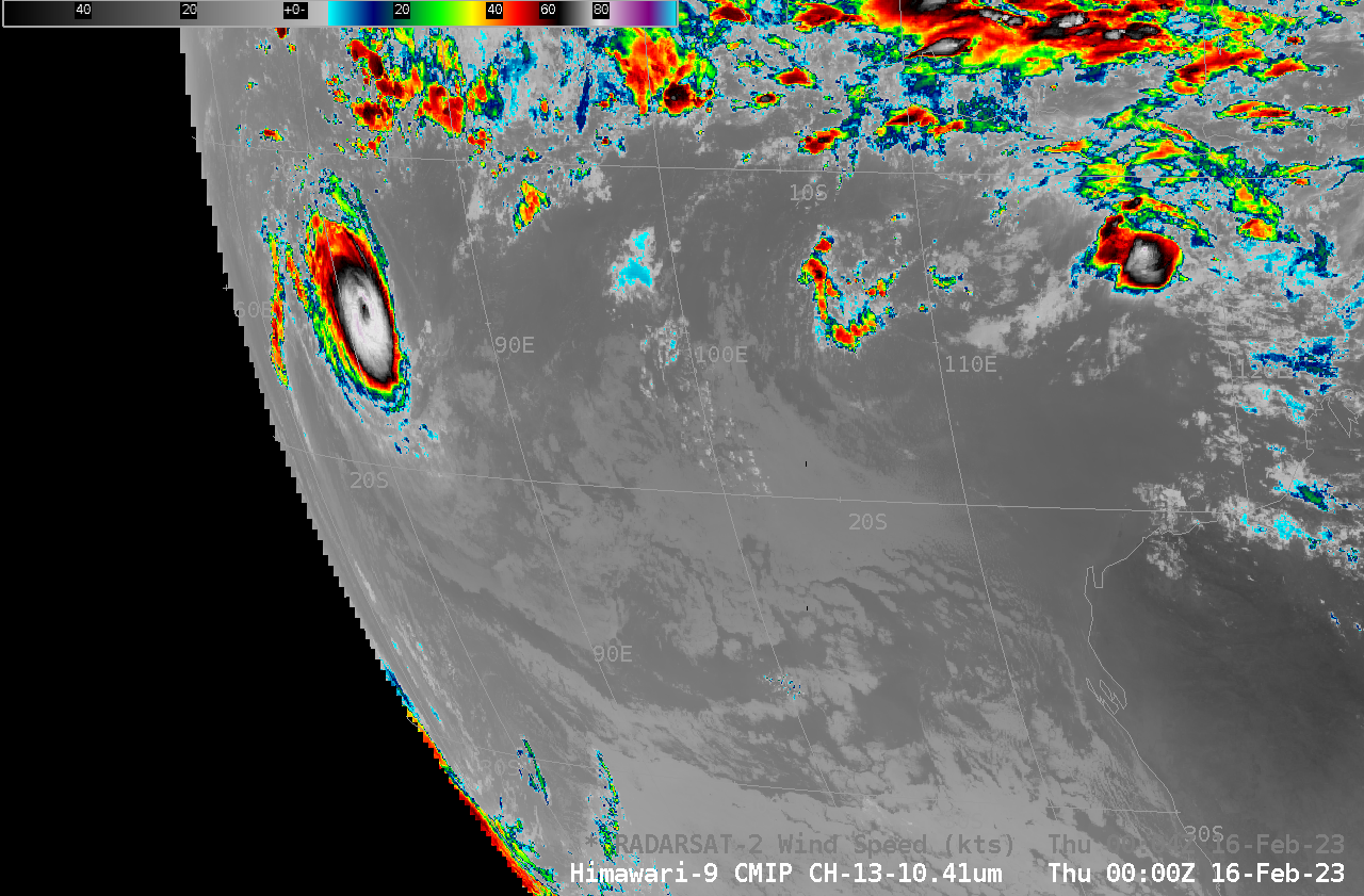
RADARSAT-2 and RCM-1 had two closely-spaced overpasses over Cyclone Freddy in the Indian Ocean early on 16 February 2023, as shown above. Eyewall speeds exceed 130 knots in the RCM-1 data! (Imagery and data are available here). The quadrant analyses for RCM-1 and for RADARSAT-2 show hurricane-force winds extending out about 40 nautical miles from the storm center. The toggle below shows 0000 UTC Himawari-9 clean window imagery overlain with the 0004 UTC RADARSAT-2 SAR Winds. Because Freddy now is almost at the limb of the Himawari-9 imagery (as shown here), there is a noticeable parallax shift in the Himawari-9 clouds — away from the sub-satellite point (for Himawari-9, that’s at 140.7o E longitude; Freddy was at 82.2o E Longitude!)
Himawari-9 Clean Window infrared (10.4 µm) imagery and RADARSAT-2 SAR winds, 0000 UTC on 16 February 2023 (Click to enlarge)
The toggle below compares 0000 UTC Clean Window imagery from Himawari-9 (AHI data) and from GEOKOMPSAT-2 (over the Equator at 128.2o E) (AMI data). The parallax shift in the AMI data is smaller than with AHI because Freddy is closer to GEOKOMPSAT-2’s subsatellite point. (Himawari HSD and Geokompsat-2 Level 1b files were processed with geo2grid software for these images). However, both satellites show an eye to the west of its SAR-derived location. Note also the degradation in Himawari-9 image acuity over the western part of the domain; brightness temperatures are also cooler over the western quarter of the domain, likely due to limb cooling (also discussed in this blog post): radiation from the edge of a Full-Disk scan (compared to radiation from the sub-satellite point) will pass through more of the colder upper troposphere (because of the much more slanted path towards the satellite) before reaching the satellite detectors, and a cooler temperature will be perceived.
Himawari-9 and Geokompsat-2 Clean Window infrared (10.4 µm and 10.5 µm, respectively) at 0000 UTC on 16 February 2023 (Click to enlarge)
Earlier SAR captures of Freddy’s eye with comparisons to Himawari-9 imagery are available here. Thanks to JMA and KMAs for the data!
The toggle below compares EWS-G1 infrared imagery (4-km resolution) with AHI data remapped to the EWS-G1 projection. Both satellites were sampling the eye near 0000 UTC on 16 February. EWS-G1 is over the equator near 66oE, so any eye displacement due to parallax will be to the east of the eye, i.e. in the opposite direction of the Himawari-9 parallax displacement.
Clean window infrared Himawari-9 imagery (10.4 µm, remapped to the EWS-G1 projection) and EWS-G1 imagery (10.8 µm), ca. 0000 UTC on 16 February 2023 (Click to enlarge)
Cyclone Freddy was at its strongest at around 0000 UTC on 16 February, as noted here.


