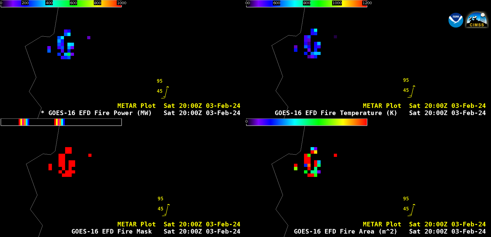
GOES-16 Fire Power (top left), Fire Temperature (top right), Fire Mask (bottom left) and Fire Area (bottom right) derived products, from 1300 UTC on 02 February to 0500 UTC on 04 February [click to play animated GIF | MP4]
All 4 components of the GOES-16 (GOES-East) Fire Detection and Characterization Algorithm (FDCA) (above) showed the diurnal variability of thermal signatures associated with a large and deadly wildfire complex near Viña del Mar and Quilpué in the Valparaíso District — located along the central coast of Chile — from 02-04 February 2024 (maximum Fire Power values occasionally reached 2200-2300 MW). After the wildfires began around 1510 UTC on 02 February, they spread northward rather quickly (due to strong southerly winds) — until an influx of cooler and more moist Pacific air early on 04 February helped to suppress the fire behavior. The METAR site plotted in the imagery is Santiago International Airport (where daytime air temperatures rose into the 90s F on 02/03 February).
A larger-scale animation of the FDCA products (below) indicated that additional wildfires were active farther to the south in Chile — with notable fires to the west of Curicó (the southernmost METAR site plotted in the imagery), which continued burning into the daytime hours on 04 February.
GOES-16 Fire Power (top left), Fire Temperature (top right), Fire Mask (bottom left) and Fire Area (bottom right) derived products, from 1300 UTC on 02 February to 0000 UTC on 05 February [click to play animated GIF | MP4]
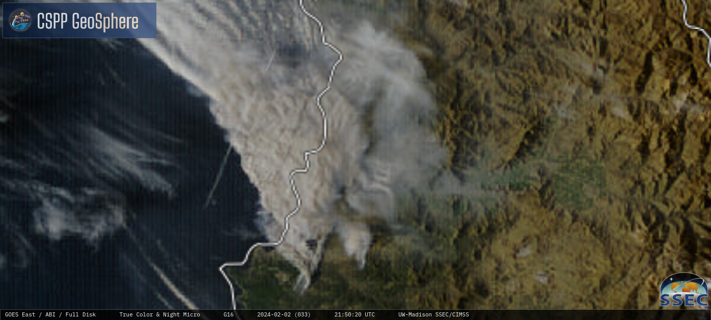
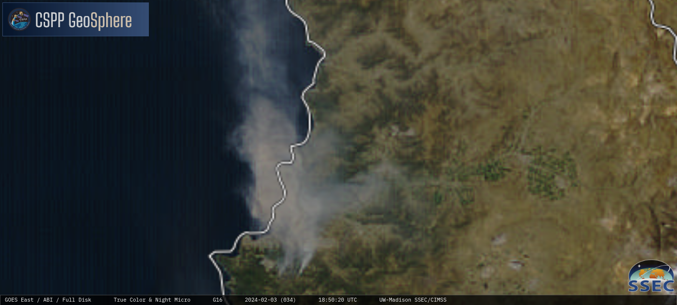
GOES-16 daytime True Color RGB and Nighttime Microphysics RGB images, from 1500 UTC on 02 February to 0700 UTC on 03 February [click to play MP4 animation]
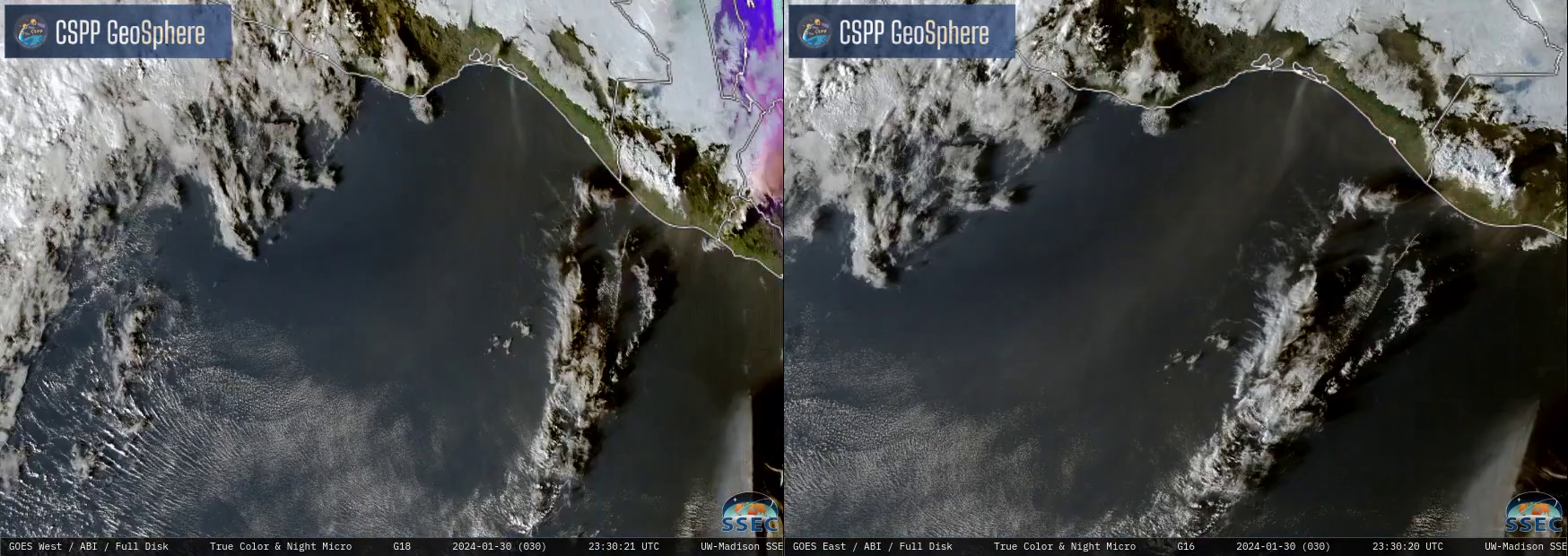
GOES-16 daytime True Color RGB and Nighttime Microphysics RGB images from the CSPP GeoSphere site revealed dense smoke plumes from the Viña del Mar and Valparaiso area that were transported northward — and clusters of hot fire pixels (darker shades of purple to blue) that persisted well after sunset — on 02 February (above) and 03 February (below).
GOES-16 daytime True Color RGB and Nighttime Microphysics RGB images, from 1300 UTC on 03 February to 0650 UTC on 04 February [click to play MP4 animation]
The four-panel animation below covers the initiation of the fires. The fire temperature RGB shows that most of the surface is red, because surface temperatures are very warm: Land Surface Temperatures from GOES-16 show values exceeding 120o F during the warmest part of the day, cooling to the mid-90s by 2300 UTC. Initiation of the fires shows up as a brighter red point that quickly turns more yellow and whitish as the fires intensify.
===== 05 February Update =====
Landsat-9 Natural Color RGB image at 1440 UTC on 05 February [click to enlarge]
A 30-meter resolution Landsat-9 Natural Color RGB image at 1440 UTC on 05 February (above) revealed the burn scar from the wildfire complex that destroyed portions of Viña de Mar and Quilpué.
View only this post Read Less

