On 20 July 2010, United Airlines Flight 967 en route from Washington Dulles to Los Angeles encountered severe turbulence over the central US, and had to divert and land at Denver to medically treat nearly 30 passengers who suffered significant injuries. The flight track diversion is shown above (courtesy of FlightAware.com).AWIPS images... Read More
")
United Airlines Flight 967 flight track diversion (courtesy of FlightAware.com)
On 20 July 2010, United Airlines Flight 967 en route from Washington Dulles to Los Angeles encountered severe turbulence over the central US, and had to divert and land at Denver to medically treat nearly 30 passengers who suffered significant injuries. The flight track diversion is shown above (courtesy of FlightAware.com).
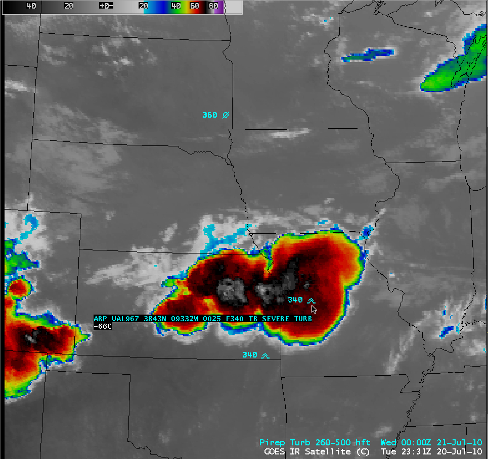
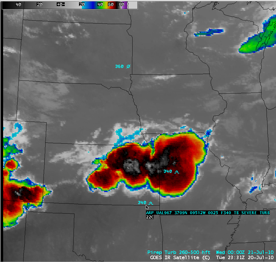
AWIPS images of 4-km resolution GOES-13 10.7 µm IR channel data (below) and GOES-13 6.5 µm water vapor channel data revealed large clusters of rapidly-developing thunderstorms over Kansas and Missouri during the afternoon and evening hours. The coldest GOES-13 cloud top IR brightness temperature was -81º C (violet color enhancement) at 22:45 UTC. However, it is unclear of the exact location of the turbulence encounter, since AWIPS plotted a SEVERE TURB report from UAL967 at Flight Level 34,000 feet over both Missouri and Kansas. Some media reports suggest that the event occurred over southwestern Missouri.

GOES-13 10.7 µm IR images + Pilot reports of turbulence
These strong thunderstorms were developing along a surface trough axis just south of a stationary frontal boundary, where the GOES-13 Sounder CAPE product indicated that the air mass was quite unstable. According to the SPC Storm Reports, there were a number of damaging wind reports associated with these thunderstorms, including surface wind gusts to 70 mph in Missouri and 80 mph in Kansas.
A comparison of 1-km resolution POES AVHRR 10.8 µm IR and 0.63 µm visible images at 22:25 UTC (below) showed cloud top IR brightness temperatures as cold as -88º C over Missouri and -90º C over Kansas (darker violet color enhancement). The visible image revealed tell-tale shadows of overshooting tops from intense updrafts.

POES AVHRR 10.8 µm IR image + 0.63 µm visible image
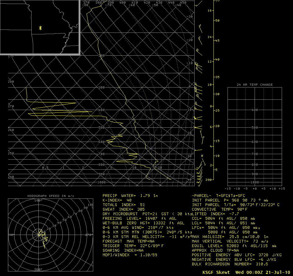
1-km resolution GOES-13 0.63 µm visible channel images (below) also showed a number of overshooting tops associated with these thunderstorms. The rawinsonde report from Springfield, Missouri indicated a maximum vertical velocity of 73 meters per second!

GOES-13 0.63 µm visible channel images + Pilot reports of turbulence
A closer view using McIDAS images of 1-km resolution GOES-15 and GOES-13 0.63 µm visible channel data (below) also shows the times of the aircraft positios as it approached the southeastern edge of the thunderstorm anvil.
 and GOES-13 (right) visible channel images (with aircraft position times)")
GOES-15 (left) and GOES-13 (right) visible channel images (with aircraft position times)
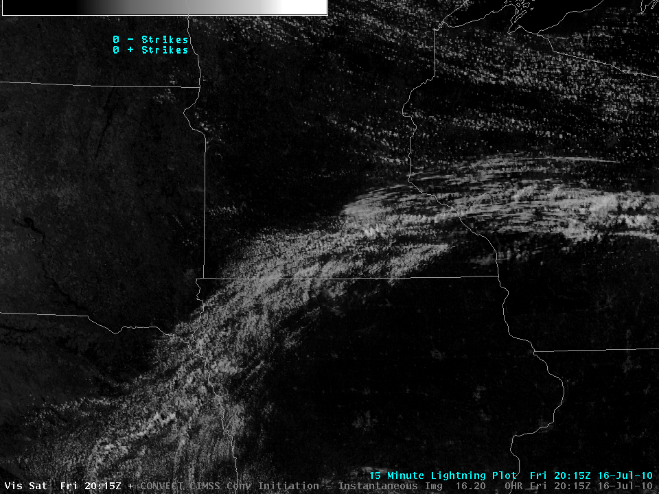
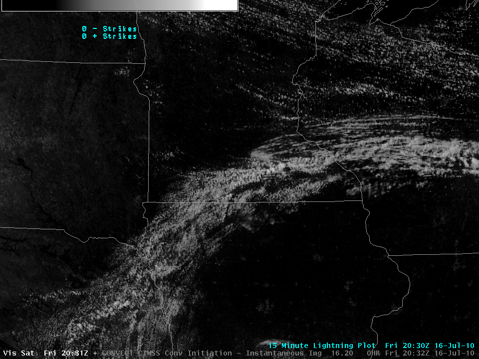
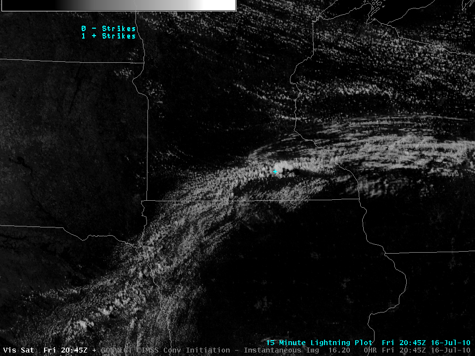
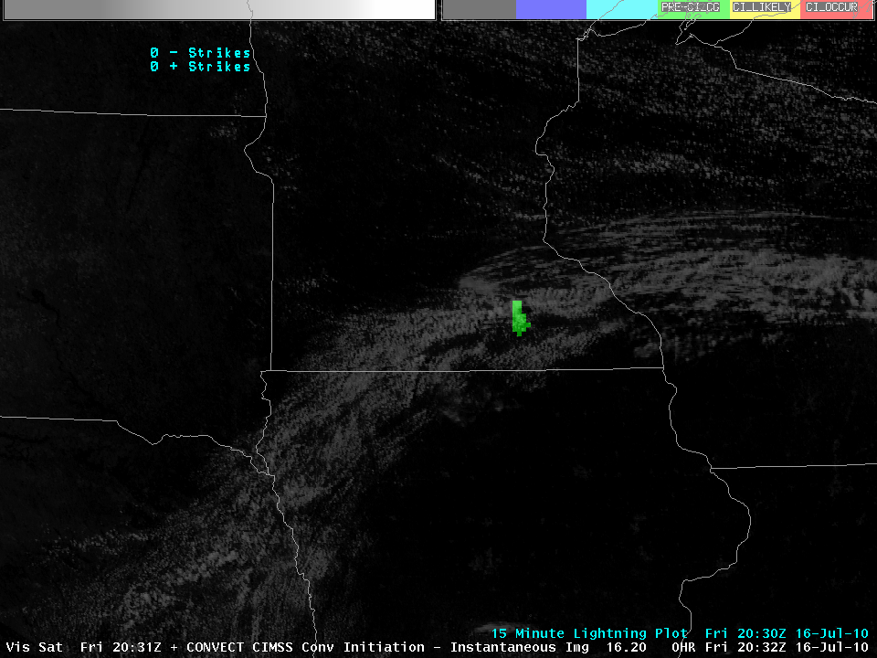
Examples of two of the SNAAP Convective Storm Monitoring and Nowcasting products (below) demonstrate the ability to use satellite data to help detect overshooting tops that might pose increased risks for turbulence.

SNAAP Overshooting Top + Turbulence Risk satellite products
An example of the NCAR Turbulence Detection Algorithm (below) showed the potential for turbulence at 36,000 feet across a large portion of Kansas and Missouri.

NCAR Turbulence Detection Algorithm
For additional satellite image analysis of this case, see the VISIT Meteorological Interpretation Blog.
View only this post
Read Less


