
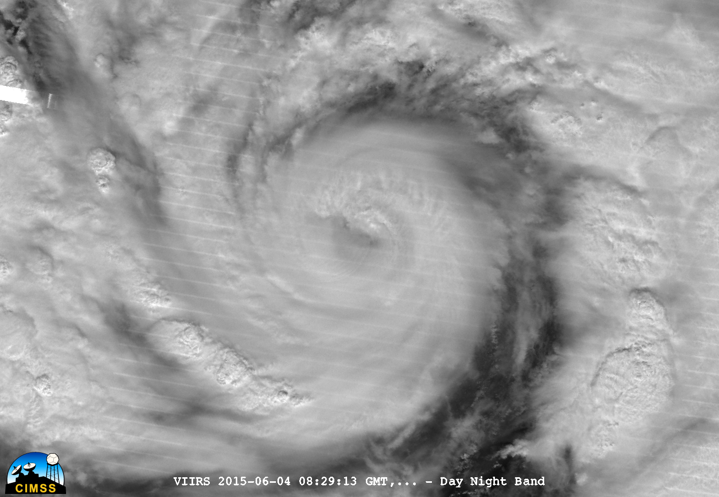
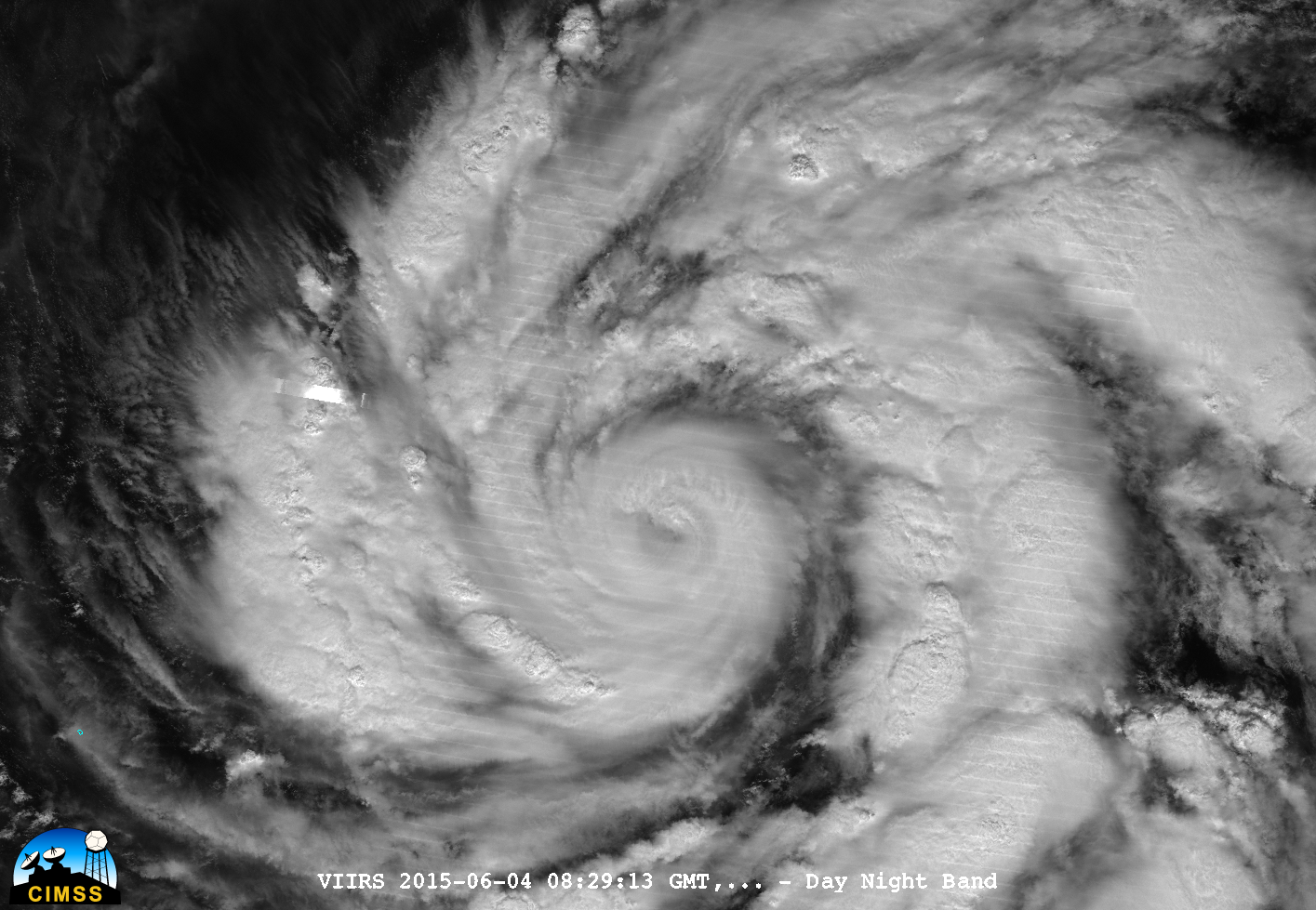
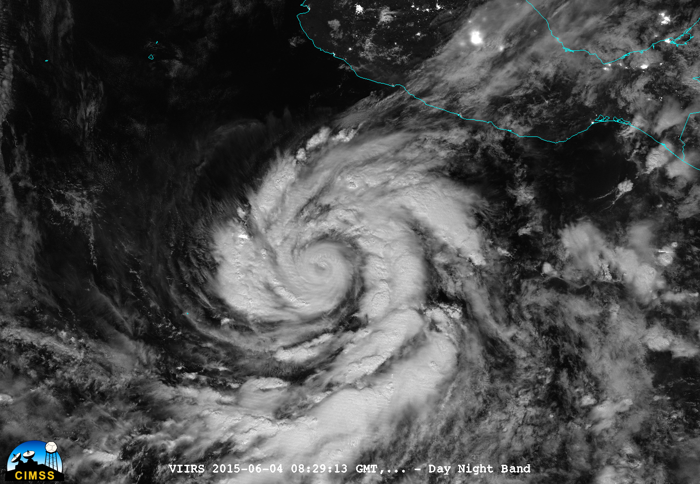
Suomi NPP overflew Hurricane Blanca early in the morning on 4 June, during a near-full Moon, and the Day Night Band imagery, above, toggled with the 11.35 µm imagery, show the hurricane. (Day/night band imagery of the eye is here, the entire storm is here, and zoomed out is here;... Read More
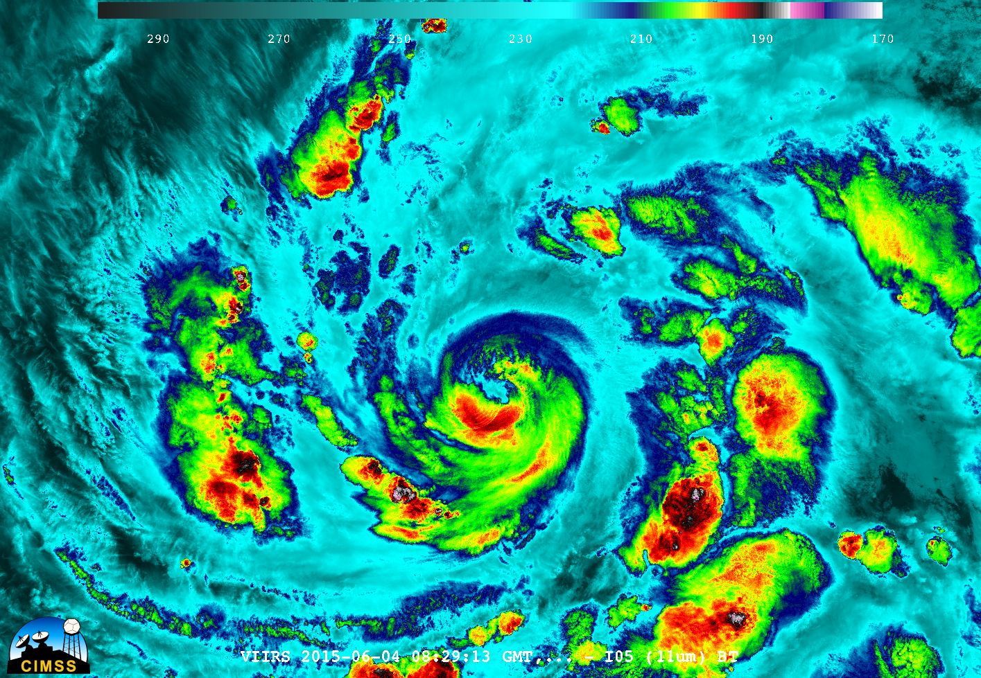
Suomi NPP VIIRS Day Night Band 0.70 µm Visible and 11.35 µm infrared imagery over Blanca, 0829 UTC 4 June 2015 (Click to enlarge)
Suomi NPP overflew Hurricane Blanca early in the morning on 4 June, during a near-full Moon, and the Day Night Band imagery, above, toggled with the 11.35 µm imagery, show the hurricane. (Day/night band imagery of the eye is here, the entire storm is here, and zoomed out is here; click for 11.35 µm imagery of the eye, the entire storm, and zoomed out). Deep convection overnight did not wrap all the way around the storm. Evidence of dry air entrained into the circulation is apparent.
GOES-15 Imager 10.7 µm infrared channel images (click to play animation)
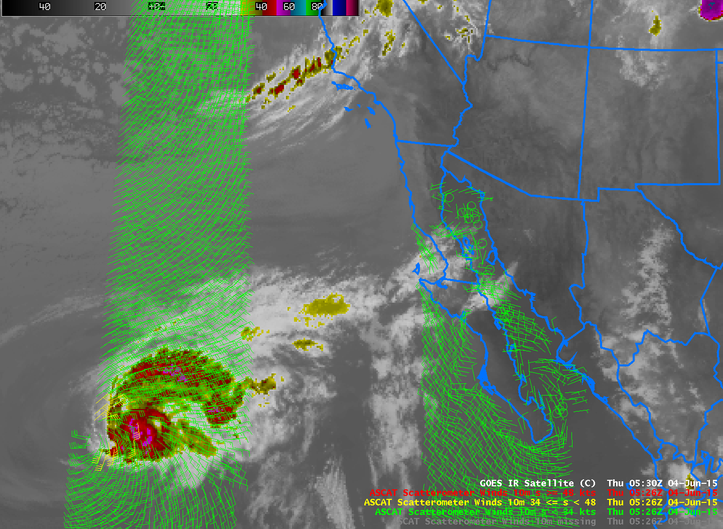
The 3-hourly animation of 10.7 micron imagery, above, from 3-4 June 2015 shows Hurricane Blanca southwest of the Mexican coast, drifting southwestward. Cold cloud tops that were apparent at the start of the loop warm by the end, perhaps because convection is being suppressed by the presence of dry air. MIMIC Total Precipitable Water (below) suggests that dry air is being entrained into Blanca’s circulation from the north. (Update on Andres, also apparent in the MIMIC Total Precipitable Water animation: This overlay of Metop ASCAT winds on top of GOES 10.7 imagery from ~0530 UTC on June 4 shows a swirl that is offset from the convection. Andres is forecast to become post-tropical later on June 4.)
MIMIC Total Precipitable Water animation for the 72 hours ending 1300 UTC on 4 June 2015 (click to enlarge)
Visible imagery from GOES-13 from June 3 and June 4, below, show a less distinct/cloudier eye on 4 June compared to 3 June. Multiple overshooting tops persist in the circulation of the system, but the coarse 30-minute temporal resolution of the imagery cannot capture the lifecycle of these quickly evolving events.
GOES-13 Imager 0.63 µm visible channel images (click to play animation)
Water vapor imagery from GOES-13 from June and June 4, below, also confirm a consistently less organized storm. The dry air penetrating from the north is apparent in the imagery, but it appears not to have entered into the circulation of the storm, at least not at levels detected by the water vapor channel.
GOES-13 Imager 6.5 µm infrared water vapor channel images (click to play animation)
Morphed Microwave Imagery (MIMIC) from this website shows the evolution of the central eye structure, below. The eyewall that was much closer to the storm center at the start of the animation has been replaced by a weaker, larger eyewall.
Morphed Microwave Imagery, 48 hours ending 1500 UTC 4 June 2015 (click to enlarge)
For more information on this storm, please visit the National Hurricane Center website or the SSEC/CIMSS Tropical Weather website.
View only this post
Read Less
