
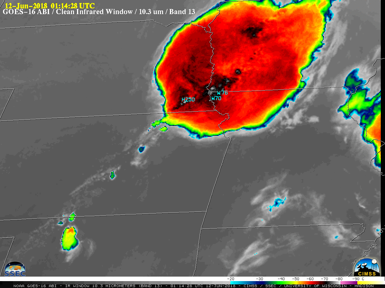
A Mesoscale Convective System (MCS) developed over eastern Nebraska early in the evening on 11 June 2018, then propagated southward across the Plains during the subsequent overnight hours. GOES-16 (GOES-East) “Clean” Infrared Window (10.3 µm) images with plots of SPC storm reports are shown above; a Mesoscale Sector was positioned over the region, providing images... Read More
GOES-16 “Clean” Infrared Window (10.3 µm) images, with plots of SPC storm reports [click to play MP4 animation]
A Mesoscale Convective System (MCS) developed over eastern Nebraska early in the evening on
11 June 2018, then propagated southward across the Plains during the subsequent overnight hours. GOES-16
(GOES-East) “Clean” Infrared Window (
10.3 µm) images with plots of
SPC storm reports are shown above; a Mesoscale Sector was positioned over the region, providing images at 1-minute intervals.
A closer look over Kansas using Infrared imagery from polar-orbiting satellites (below) revealed some very cold cloud-top infrared brightness temperatures, which included -87ºC on MODIS, -90ºC on VIIRS and -92ºC on AVHRR.
![POES AVHRR, Terra/Aqua MODIS and Suomi NPP VIIRS Infrared images, with plots of SPC storm reports [click to enlarge]](https://cimss.ssec.wisc.edu/satellite-blog/wp-content/uploads/sites/5/2018/06/180612_avhrr_modis_viirs_infrared_spc_storm_reports_Plains_MCS_anim.gif)
Metop-B AVHRR, Terra/Aqua MODIS and Suomi NPP VIIRS Infrared images, with plots of SPC storm reports [click to enlarge]
The coldest air temperature on 00 UTC
rawinsonde data from Dodge City and Topeka, Kansas
(below) was -69.5ºC (at altitudes of 14.6 km/49,900 feet at Dodge City, and 17.6 km/57,700 feet at Topeka) — so in theory air parcels and cloud material within a vigorous overshooting top could have ascended a few km (or thousands of feet) beyond those altitudes to exhibit an infrared brightness temperature of -92ºC.
![Plots of rawinsonde data from Dodge City and Topeka, Kansas [click to enlarge]](https://cimss.ssec.wisc.edu/satellite-blog/wp-content/uploads/sites/5/2018/06/180612_00UTC_KDDC_KTOP_RAOBS.GIF)
Plots of rawinsonde data from Dodge City and Topeka, Kansas [click to enlarge]
A toggle between re-mapped versions of the GOES-16 ABI and Metop-B AVHRR Infrared imagery over Kansas at the time of the very cold cloud-top infrared brightness temperature
(below) revealed 2 important points: (1) with improved spatial resolution
(1 km for AVHRR, vs 2 km *at satellite sub-point* for ABI) the instrument detectors sensed much colder temperatures (
-92.6ºC with AVHRR vs
-81.2ºC with ABI), and (2) due to
parallax. the GOES-16 image features are displaced to the northwest. In addition to the isolated cold overshooting top in south-central Kansas, note the pronounced
enhanced-V storm top signature in far northeastern Kansas.
![Comparison of GOES-16 ABI and Metop-B AVHRR Infrared images [click to enlarge]](https://cimss.ssec.wisc.edu/satellite-blog/wp-content/uploads/sites/5/2018/06/180612_0336utc_goes16_metopb_infrared_Kansas_anim.gif)
Comparison of GOES-16 ABI and Metop-B AVHRR Infrared images [click to enlarge]
.
View only this post
Read Less
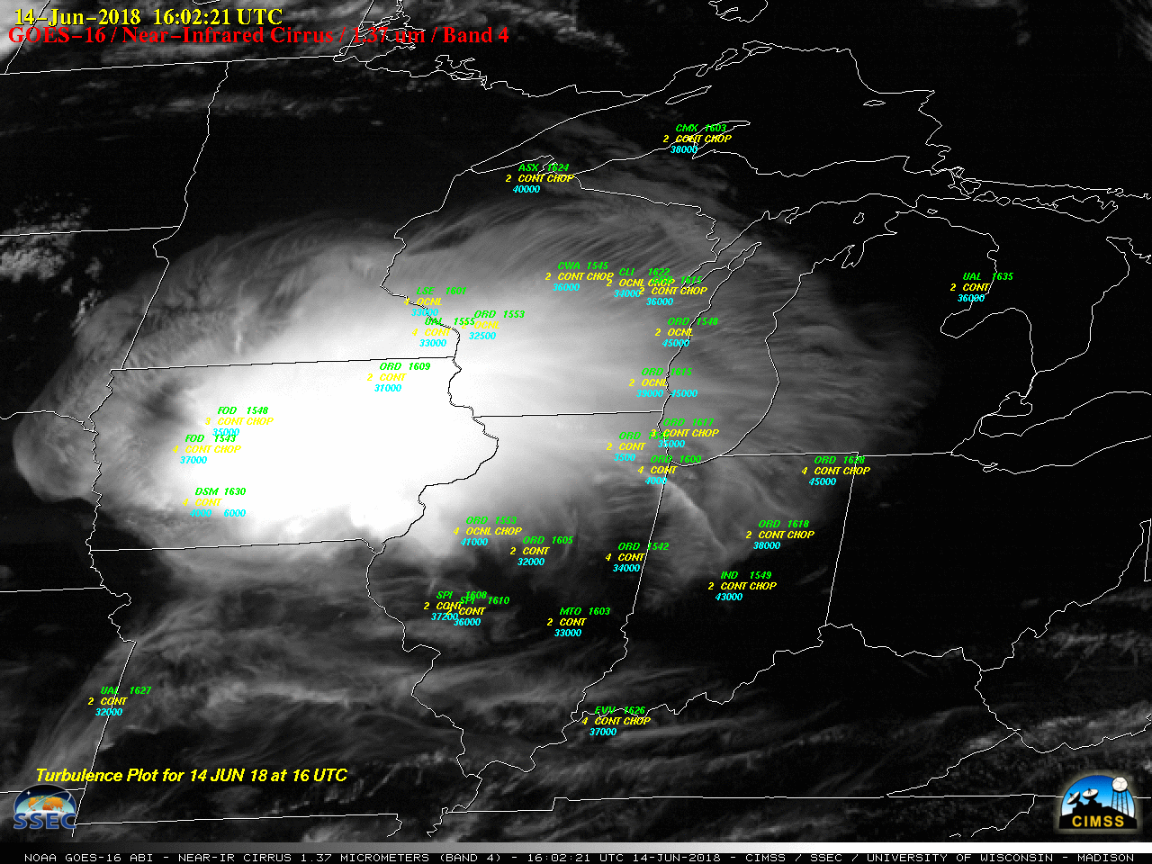


![GOES-16 Mid-level Water Vapor (6.9 µm) images, with hourly plots of turbulence [click to play MP4 animation]](https://cimss.ssec.wisc.edu/satellite-blog/wp-content/uploads/sites/5/2018/06/G16_WV_MIDWEST_TURB_14JUN2018_960x1280_B9_2018165_160221_0001PANEL_00049.GIF)
![GOES-16 "Clean" Infrared Window (10.3 µm) images, with hourly plots of turbulence [click to play MP4 animation]](https://cimss.ssec.wisc.edu/satellite-blog/wp-content/uploads/sites/5/2018/06/G16_IR_MIDWEST_TURB_14JUN2018_960x1280_B13_2018165_160221_0001PANEL_00049.GIF)

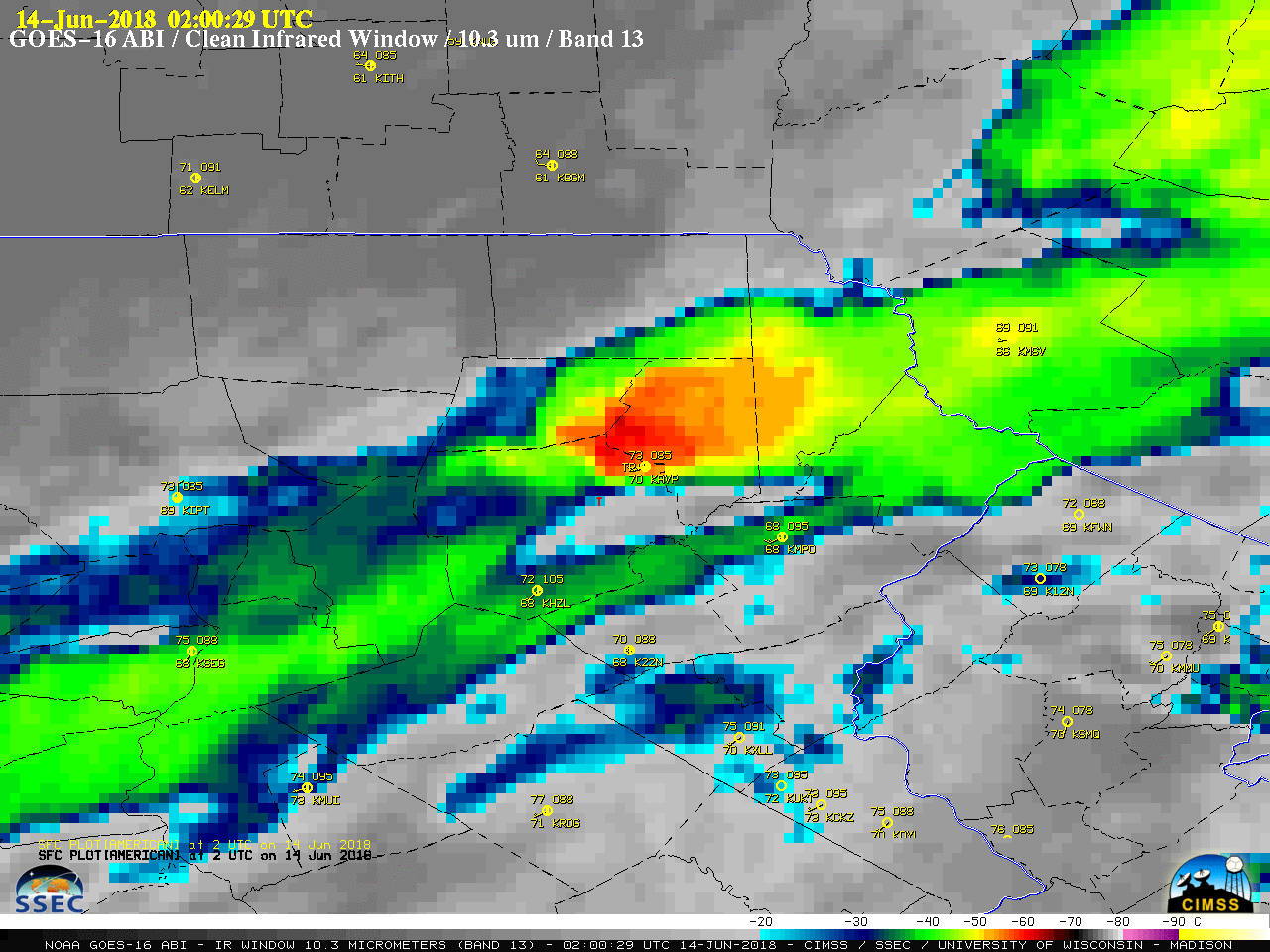
![GOES-16 Band 13 (Clean Infrared Window, 10.3 µm) images, with SPC storm reports plotted in red [click to animate]](https://cimss.ssec.wisc.edu/satellite-blog/wp-content/uploads/sites/5/2018/06/180613_goes16_infrared_spc_storm_reports_PA_svr_anim.gif)
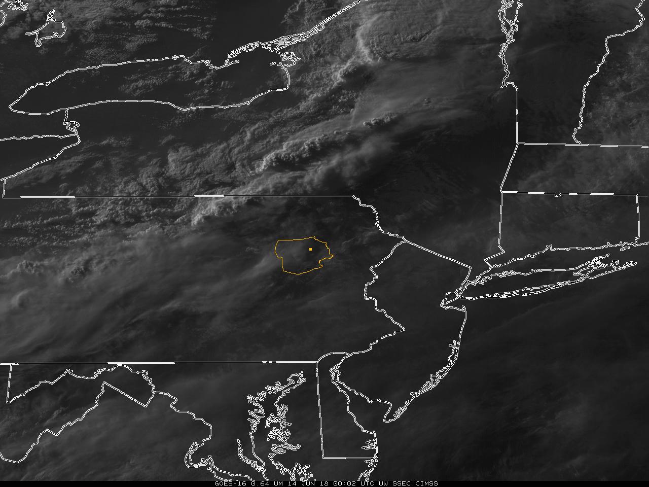
![Terra MODIS Band 31 (Infrared Window, 11.0 µm) image, with plots of cumulative SPC storm reports and the 03 UTC position of the surface cold front [click to enlarge]](https://cimss.ssec.wisc.edu/satellite-blog/wp-content/uploads/sites/5/2018/06/MODIS_IR_20180614_0221.png)

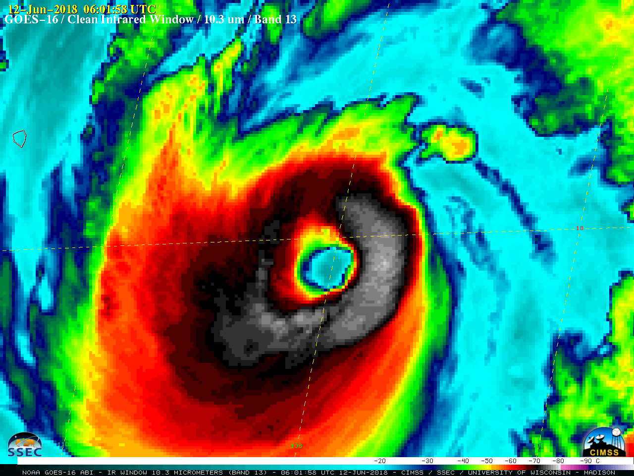
![GOES-16 "Red" Visible (0.64 µm, left) and "Clean" Infrared Window (10.3 µm, right) images [click to play MP4 animation]](https://cimss.ssec.wisc.edu/satellite-blog/wp-content/uploads/sites/5/2018/06/G16_VIS_IR_BUD_12JUN2018_958x638_B213_2018163_160358_0002PANELS_00189.GIF)
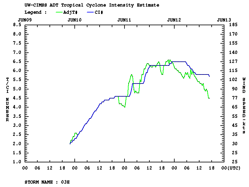
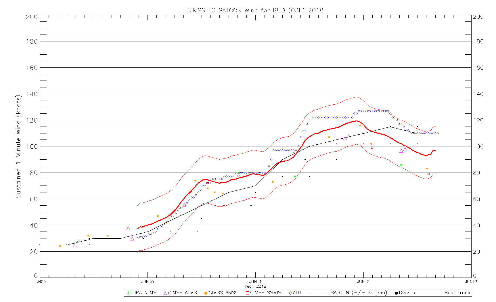
![Ocean Heat Content and Sea Surface Temperature analyses, with the track of Hurricane Bud ending at 12 UTC on 12 June [click to enlarge]](https://cimss.ssec.wisc.edu/satellite-blog/wp-content/uploads/sites/5/2018/06/180612_ohc_sst_Bud_anim.gif)
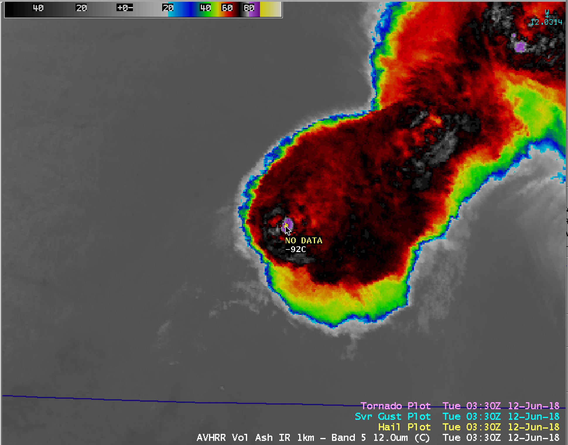
![DMSP-16 SSMIS Microwave (85 GHz) image [click to enlarge]](https://cimss.ssec.wisc.edu/satellite-blog/wp-content/uploads/sites/5/2018/06/180612_1105utc_dmsp16_ssmis_Bud.jpeg)
