GOES-15 (GOES-West) Infrared Window (10.7 µm) images (above) showed the formation of a well-defined eye of Hurricane Walaka during a period of rapid intensification (ADT | SATCON) from 0000-2330 UTC on 01 October 2018; Walaka was classified a Category 5 hurricane as of the 02 October 00 UTC advisory. Walaka was moving... Read More
![GOES-15 Infrared Window (10.7 µm) images [click to play animation | MP4]](https://cimss.ssec.wisc.edu/satellite-blog/wp-content/uploads/sites/5/2018/10/G15_IR_WALAKA_01OCT2018_960x1280_B4_2018274_220000_0001PANEL_00079.GIF)
GOES-15 Infrared Window (10.7 µm) images [click to play animation | MP4]
GOES-15 (GOES-West) Infrared Window (10.7 µm) images
(above) showed the formation of a well-defined eye of
Hurricane Walaka during a period of rapid intensification (
ADT |
SATCON) from 0000-2330 UTC on 01 October 2018; Walaka was classified a
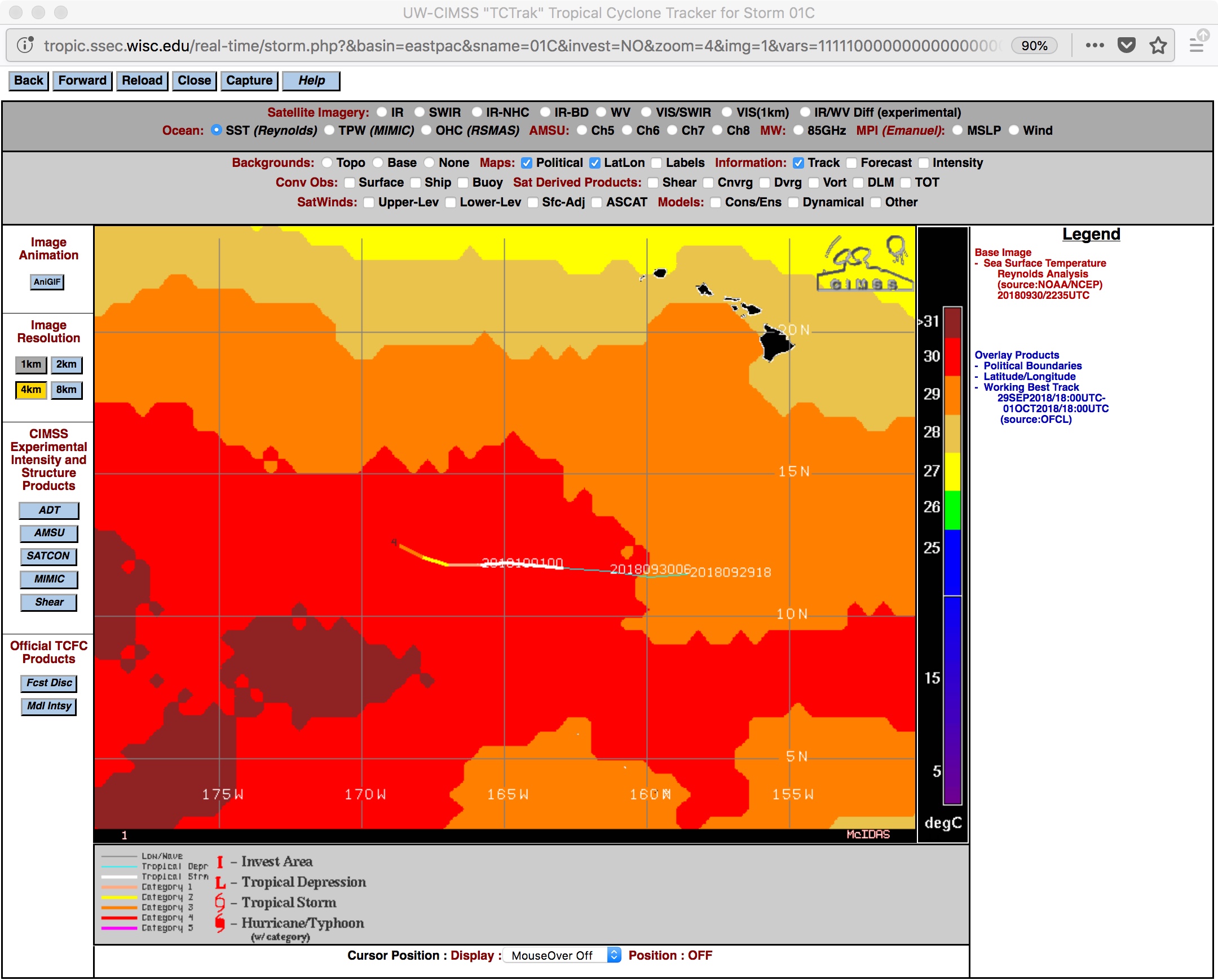
Category 5 hurricane as of the 02 October 00 UTC advisory. Walaka was moving over very warm water with
Sea Surface Temperatures of 30ºC.
A 1536 UTC DMSP-16 SSMIS Microwave (85 GHz) image from the CIMSS Tropical Cyclones site (below) revealed a small eye (reported to be 20 nautical miles in diameter at 21 UTC).
![DMSP-16 SSMIS (85 GHz) Microwave image [click to enlarge]](https://cimss.ssec.wisc.edu/satellite-blog/wp-content/uploads/sites/5/2018/10/181001_1536utc_dmsp16_ssmis_microwave_Walaka.jpeg)
DMSP-16 SSMIS (85 GHz) Microwave image [click to enlarge]
A side-by-side comparison of
JMA Himawari-8 and GOES-15 Infrared Window images
(below) showed Walaka from 2 different satellite perspectives — the superior spatial resolution of Himawari-8
(2 km, vs 4 km for GOES-15) was offset by the much larger viewing angle. Cloud-top infrared brightness temperatures were -80ºC and colder (shades of violet) from both satellites early in the animation, but warmed somewhat into the -70 to -75ºC range by 00 UTC on 02 October.
![Infrared Window images from Himawari-8 (10.3 µm, left) and GOES-15 (10.7 µm, right) [click to play animation | MP4]](https://cimss.ssec.wisc.edu/satellite-blog/wp-content/uploads/sites/5/2018/10/HIM08_G15_IR_WALAKA_01OCT2018_960x640_B134_2018274_221000_0002PANELS_00122.GIF)
Infrared Window images from Himawari-8 (10.3 µm, left) and GOES-15 (10.7 µm, right) [click to play animation | MP4]
===== 02 October Update =====
![NOAA-20 VIIRS Day/Night Band (0.7 µm) and Infrared Window (11.45 µm) images [click to enlarge]](https://cimss.ssec.wisc.edu/satellite-blog/wp-content/uploads/sites/5/2018/10/181002_1240utc_noaa20_viirs_DayNightBand_InfraredWindow_Walaka_anim.gif)
NOAA-20 VIIRS Day/Night Band (0.7 µm) and Infrared Window (11.45 µm) images [click to enlarge]
Walaka remained classified as a Category 5 hurricane until the 15 UTC advisory on 02 October, when it was assigned Category 4 status after some weakening as a result of an overnight eyewall replacement cycle. A toggle between NOAA-20 VIIRS Day/Night Band (0.7 µm) and Infrared Window (11.45 µm) images
(above; courtesy of William Straka, CIMSS) showed the storm at 1240 UTC or 2:40 am local time.
GOES-15 Infrared Window (10.7 µm) images (below) showed the northward motion of Waleka. Given that the storm was forecast to pass very close to Johnston Atoll, the US Coast Guard was dispatched to evacuate personnel on Johnston Island.
![GOES-15 Infrared Window (10.7 µm) images; the white circle shows the location of Johnston Atoll [click to play animation | MP4]](https://cimss.ssec.wisc.edu/satellite-blog/wp-content/uploads/sites/5/2018/10/G15_IR_WALAKA_02OCT2018_960x1280_B4_2018275_143000_0001PANEL_00030.GIF)
GOES-15 Infrared Window (10.7 µm) images; the white circle shows the location of Johnston Atoll [click to play animation | MP4]
The
MIMIC-TC product
(below) showed the eyewall replacement cycle during the 0000-1445 UTC period.
![MIMIC-TC morphed microwave product [click to play animation]](https://cimss.ssec.wisc.edu/satellite-blog/wp-content/uploads/sites/5/2018/10/181002_0515utc_mimic_tc_Walaka.jpeg)
MIMIC-TC morphed microwave product [click to play animation]
Around 1830 UTC, a toggle between GOES-15 Infrared (10.7 µm) and GPM GMI Microwave (85 GHz) images
(below) showed a small eye, with evidence of a larger outer eyewall suggesting that another eyewall replacement cycle was taking place.
![GOES-15 Infrared Window (10.7 µm) and GPM GMI Microwave (85 GHz) images [click to enlarge]](https://cimss.ssec.wisc.edu/satellite-blog/wp-content/uploads/sites/5/2018/10/181002_1830utc_goes15_infrared_gpm_microwave_Walaka_anim.gif)
GOES-15 Infrared Window (10.7 µm) and GPM GMI Microwave (85 GHz) images [click to enlarge]
View only this post
Read Less
![GOES-16 "Clean" Infrared Window (10.3 µm) images, 25 September - 02 October [click to play MP4 animation]](https://cimss.ssec.wisc.edu/satellite-blog/wp-content/uploads/sites/5/2018/10/G16_IR_ROSA_ZOOM_25SEP_02OCT2018_960x1280_B13_2018270_204534_0001PANEL_00216.GIF)
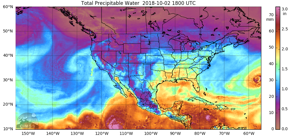
![MIMIC Total Precipitable Water product, 25 September - 02 October [click to play MP4 animation | MP4]](https://cimss.ssec.wisc.edu/satellite-blog/wp-content/uploads/sites/5/2018/10/180925_181002_mimic_tpw_Rosa_anim.gif)
![Plots of rawinsonde data from Tucson, Arizona 30 September - 02 October [click to enlarge]](https://cimss.ssec.wisc.edu/satellite-blog/wp-content/uploads/sites/5/2018/10/180930_181002_ktwc_raobs_anim.gif)
![GOES-15 Infrared Window (10.7 µm) images [click to play animation | MP4]](https://cimss.ssec.wisc.edu/satellite-blog/wp-content/uploads/sites/5/2018/10/181001_goes15_infrared_Walaka_anim.gif)
![Infrared Window images from Himawari-8 (10.3 µm, left) and GOES-15 (10.7 µm, right) [click to play animation | MP4]](https://cimss.ssec.wisc.edu/satellite-blog/wp-content/uploads/sites/5/2018/10/181001_himawari8_goes15_infrared_Walaka_anim.gif)
![GOES-15 Infrared Window (10.7 µm) images; the white circle shows the location of Johnston Atoll [click to play animation | MP4]](https://cimss.ssec.wisc.edu/satellite-blog/wp-content/uploads/sites/5/2018/10/181002_goes15_infrared_Walaka_anim.gif)
![MIMIC-TC morphed microwave product [click to play animation]](https://cimss.ssec.wisc.edu/satellite-blog/wp-content/uploads/sites/5/2018/10/181002_0000_1445utc_mimic_tc_Walaka_anim.gif)
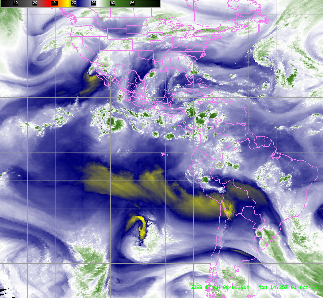


![GOES-17 Mid-level Water Vapor (6.9 µm) images [click to play MP4 animation]](https://cimss.ssec.wisc.edu/satellite-blog/wp-content/uploads/sites/5/2018/10/G17_FD_WV_B9_01OCT2018_960x1280_2018274_120522_0001PANEL_00146.GIF)
![GOES-17 "Red" Visible (0.64 µm) images [click to play MP4 animation]](https://cimss.ssec.wisc.edu/satellite-blog/wp-content/uploads/sites/5/2018/10/G17_FD_VIS_SOAM_SUNGLINT_01OCT2018_960x1280_B2_2018274_124522_0001PANEL_00010.GIF)
![NOAA-20 and Suomi NPP VIIRS Day/Night Band (0.7 µm) images [click to enlarge]](https://cimss.ssec.wisc.edu/satellite-blog/wp-content/uploads/sites/5/2018/09/180928_0018utc_noaa20_0108utc_suomiNPP_viirs_DayNightBand_Medicane_anim.gif)
![Meteosat-11 Visible (0.8 µm) images, with hourly plots of wind barbs (yellow) and wind gusts (red) [click to play animation | MP4]](https://cimss.ssec.wisc.edu/satellite-blog/wp-content/uploads/sites/5/2018/09/180928_meteosat11_visible_winds_gusts_Medicane_anim.gif)
![Meteosat-11 Visible (0.8 µm) images, with hourly plots of winds (yellow) and gusts in knots (red) [click to play animation | MP4]](https://cimss.ssec.wisc.edu/satellite-blog/wp-content/uploads/sites/5/2018/09/180929_meteosat11_visible_winds_gusts_Medicane_anim.gif)
![Terra/Aqua MODIS True Color RGB images on 28 and 29 September [click to enlarge]](https://cimss.ssec.wisc.edu/satellite-blog/wp-content/uploads/sites/5/2018/09/180928_180929_terra_aqua_modis_truecolor_Medicane_anim.gif)
![MIMIC morphed Total Precipitable Water images, 27-29 September [click to play animation | MP4]](https://cimss.ssec.wisc.edu/satellite-blog/wp-content/uploads/sites/5/2018/09/180927_180929_mimic_tpw_Medicane_anim.gif)
