
GOES-17 Band 10 (7.34 µm) imagery, 0900-1700 UTC on 13 February 2018 (Click to animate)
(The Experimental GOES-17 Data Fusion link is here).
GOES-17 is now operational as GOES-West at 137.2º W Longitude, as noted here and elsewhere. However, Loop Heat Pipe (LHP) problems persist (as noted here and here and here), with the effect varying seasonally. Because of the Loop Heat Pipe malfunction, the Advanced Baseline Imager warms up, emitting radiation at wavelengths similar to those being sensed from the Earth. This does not happen during the day when the ABI instrument is pointing towards the Earth and the Sun is behind the satellite. During the night, however, the sun illuminates the ABI instrument and warms it. This effect is most noticeable (and detrimental to the imagery) around the solstices. The animation above shows the effects of the Loop Heat Pipe on Band 10, the low-level water vapor imagery. Starting at about 1015 UTC, there is a perceptible warming of the image, globally, shortly after that the image integrity is lost and the data become unuseable. At 1615-1630 UTC, the instrumentation cools enough to produce, again, useable imagery.
The chart below shows how the temperature of the focal plane in the ABI changes throughout the course of the year. The differences between Northern Hemisphere Vernal and Autumnal Equinoxes occur because the Earth is closer to the Sun at the Northern Hemisphere Vernal Equinox. The chart also shows the effects of ‘Eclipse’ — when the satellite moves through the Earth’s shadow. When the ABI is in the Earth’s shadow, it is not being heated by the Sun (and that’s why the GOES-R Series carries batteries to power the satellite at that time). The reduced heating occurs between 26 February and 14 April in the Spring, and between 30 August and 16 October in the Fall. The chart also contains for the longwave infrared bands the temperature at which the heat from the satellite increases the likelihood of bad data.
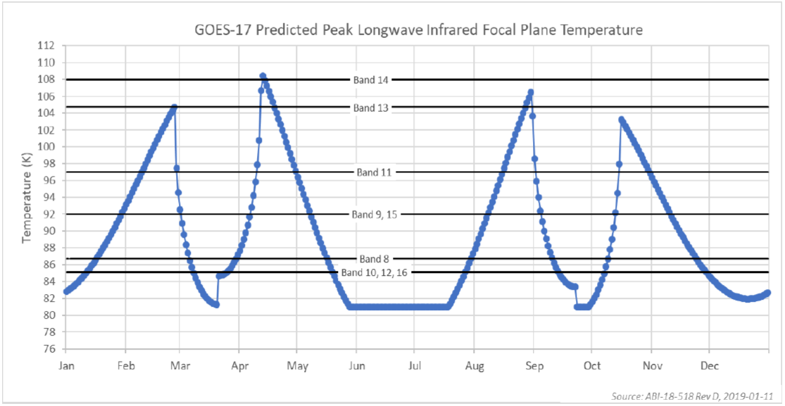
Warmest Focal Plane Temperature as a function of Year. Also included: the threshold temperatures when the ABI Detection is affected by the warmer Focal Plane. The step in values near both Equinoxes occurs when a Yaw Flip is performed on the satellite (Click to enlarge)
Note in the plot above that Band 13 and Band 14, the clean window and longwave infrared window bands at 10.3 µm and 11.2 µm, respectively, is relatively unaffected by warming. This 10.3 µm animation (spanning the same times as the animation above) shows subtle features that are related to warming because of the faulty Loop Heat Pipe, but overall, data integrity is preserved.
The GOES-17-only fusion solution for mitigating data outages uses GOES-17 ABI Clean Window (10.3 µm) radiances to create missing spectral band radiances. In this method, the last full set of calibrated radiances at time t0 is marked (For GOES-17 at present this is done at 0900 UTC). Then, for subsequent times when LHP issues cause missing data, a so-called k-d tree search (discussed in this paper: Weisz, E., B. A. Baum, and W. P. Menzel, 2017: Construction of high spatial resolution narrowband infrared radiances from satellite-based imager and sounder data fusion. J. Appl. Remote Sens. 11 (3), 036022, doi: 10.1117/1.JRS.11.036022) is performed on time t0 infrared window band 13 measurements to find the five t0 pixels that best match each time t infrared window band 13 pixel; the five k-d tree time t0 matches for each pixel are then averaged for all ABI IR spectral bands to estimate ABI bands at time t for that pixel.
In other words, the fusion method (1) finds the five best matches of time t0 Band 13 measurements for each time t Band 13 measurement and then (2) uses the average of those t0 matches for each missing spectral band to create a fusion estimate at time t. Using time 0900 UTC for t0, when Loop Heat Pipe issues subsequently impact data quality, the Band 13 image at that time is used to predict what the other bands would look like — based on the relationship established for Band 13 measurements between time t and time t0 at 0900 UTC. The fusion method is most challenging for the Band 10 imagery — because it is the least correlated with Band 13 (especially in regions of clear skies). In contrast, a window channel like Band 11 is highly correlated with Band 13 and the Data Fusion product has few artifacts. This animation compares Band 13 and Band 11 — very similar! — and Band 13 and Band 10 — not that similar, except in regions of clouds.
A resultant image is shown below. The left-most image is the unusable GOES-17 Band 10 image. The middle image shows the GOES-17 water vapor image produced via data fusion; the right-most image is the corresponding GOES-16 Band 10 image over the same region (a region that is midway between the two satellite nadirs so that view angle differences are minimized). There are some subtle differences; in particular the Fusion product shows values that are cooler than GOES-16 in some regions, but the qualitative aspects of the match are good.
(The GOES-17 Imagery below pre-dates the 1800 UTC 12 February 2019 time when GOES-17 became operational and should therefore be considered preliminary and non-operational)
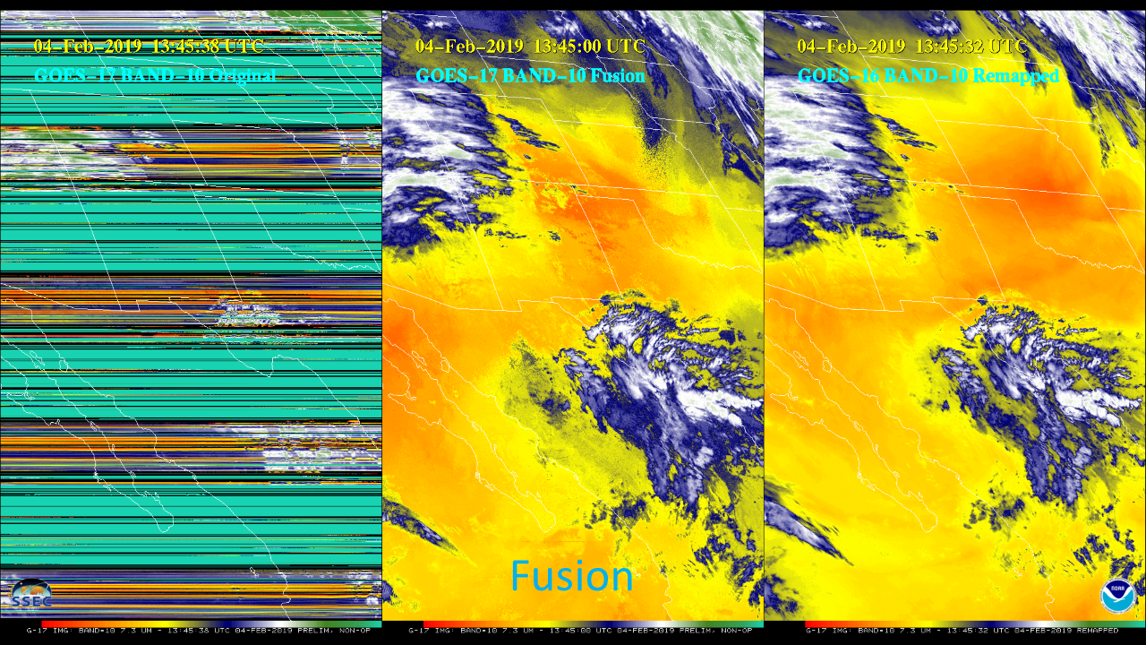
GOES-17, GOES-17 Data Fusion, and GOES-16 Low-Level Water Vapor (Band 10, 7.3 µm) Imagery, 1300 – 1445 UTC on 4 February 2019 (Click to play mp4 animation)
Data Fusion Imagery is available at the SSEC Geo Browser (Link). It is a separate drop-down menu (‘GOES-17 Fusion’) and should be considered experimental. The animation below shows the transition between non-fusion and fusion data. Here is a full-disk animation from 13 February (1200 UTC to 1700 UTC) that shows Fusion Data transitioning back to GOES-17 data as the Loop Heat Pipe issues end in the morning.

GOES-17 Low-Level water vapor imagery (7.3 µm) at 1100, 1115 and 1130 UTC. Data Fusion was used to produce the 1130 UTC image (Click to enlarge)
View only this post Read Less
![Visible images, centered at Seattle, from (left to right) GOES-17, GOES-15, GOES-16 and GOES-13 [click to play animation | MP4]](https://cimss.ssec.wisc.edu/satellite-blog/wp-content/uploads/sites/5/2019/02/190213_goes17_goes15_goes16_goes13_visible_Seattle_anim.gif)
![GOES-13 Visible (0.63 µm), Shortwave Infrared (3.9 µm), Water Vapor (6.5 µm), Infrared Window (10.7 µm) and Infrared CO2 Absorption (13.3 µm) images at 2015 UTC [click to enlarge]](https://cimss.ssec.wisc.edu/satellite-blog/wp-content/uploads/sites/5/2019/02/190213_2115utc_goes13_fullDisk_anim.gif)


![GOES-17 Mid-level Water Vapor (6.9 µm) images [click to play animation | MP4]](https://cimss.ssec.wisc.edu/satellite-blog/wp-content/uploads/sites/5/2019/02/190212_goes17_full_disk_waterVapor_anim.gif)
![GOES-17 images from the 16 ABI spectral bands, centered on the Big Island of Hawai'i [click to play animation | MP4]](https://cimss.ssec.wisc.edu/satellite-blog/wp-content/uploads/sites/5/2019/02/190212_goes17_16spectralBands_HI_anim.gif)
![Image loop that cycles through all 16 ABI Bands from GOES-17, covering most of Alaska [click to play MP4 animation]](https://cimss.ssec.wisc.edu/satellite-blog/wp-content/uploads/sites/5/2019/02/ak_band02-20190212_221537.png)
![GOES-17 + GOES-16 Infrared (11.2 µm) images [click to play animation | MP4]](https://cimss.ssec.wisc.edu/satellite-blog/wp-content/uploads/sites/5/2019/02/190212_goes17_goes16_infrared_anim.gif)
![Sequence of GOES-17 Band 09 (6.9 µm Water Vapor) images during a spike in the Focal Plane Module temperature on 11 February 2019 [click to enlarge]](https://cimss.ssec.wisc.edu/satellite-blog/wp-content/uploads/sites/5/2019/02/190211_goes17_band9_fpm_anim.gif)
![Sequence of GOES-17 CONUS sector Band 09 (6.9 µm Water Vapor) images during a spike in the Focal Plane Module temperature on 11 February 2019 [click to enlarge]](https://cimss.ssec.wisc.edu/satellite-blog/wp-content/uploads/sites/5/2019/02/190211_goes17_band9_fpm_conus_anim.gif)
