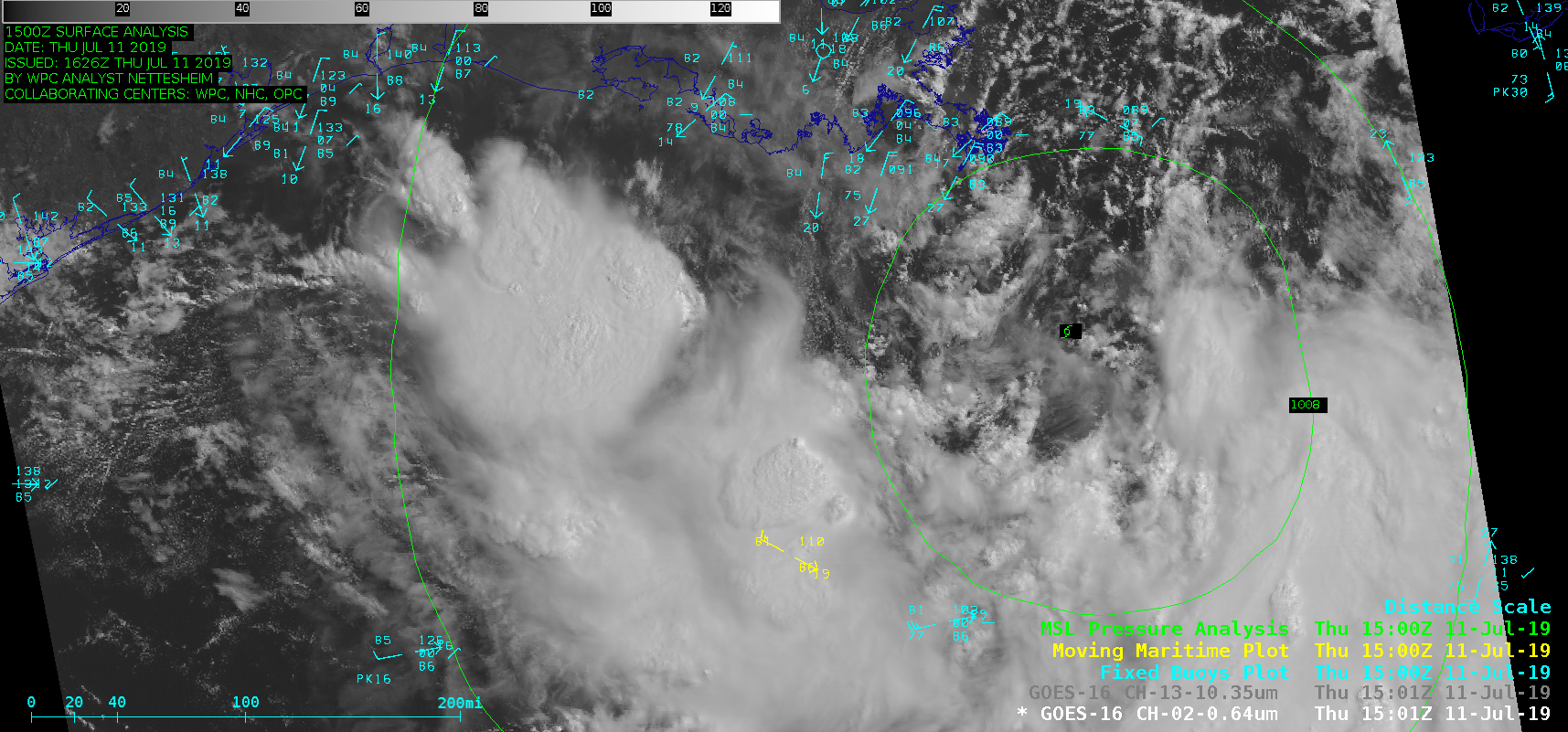
Tropical Storm Barry formed in the far northern Gulf of Mexico on 11 July 2019 — 1-minute Mesoscale Domain Sector GOES-16 (GOES-East) “Red” Visible (0.64 µm) and “Clean” Infrared Window (10.35 µm) images (above) displayed increasing convection associated with the tropical cyclone. The coldest cloud-top infrared brightness temperatures were -86ºC.As was seen in an animation of GOES-16 Infrared... Read More
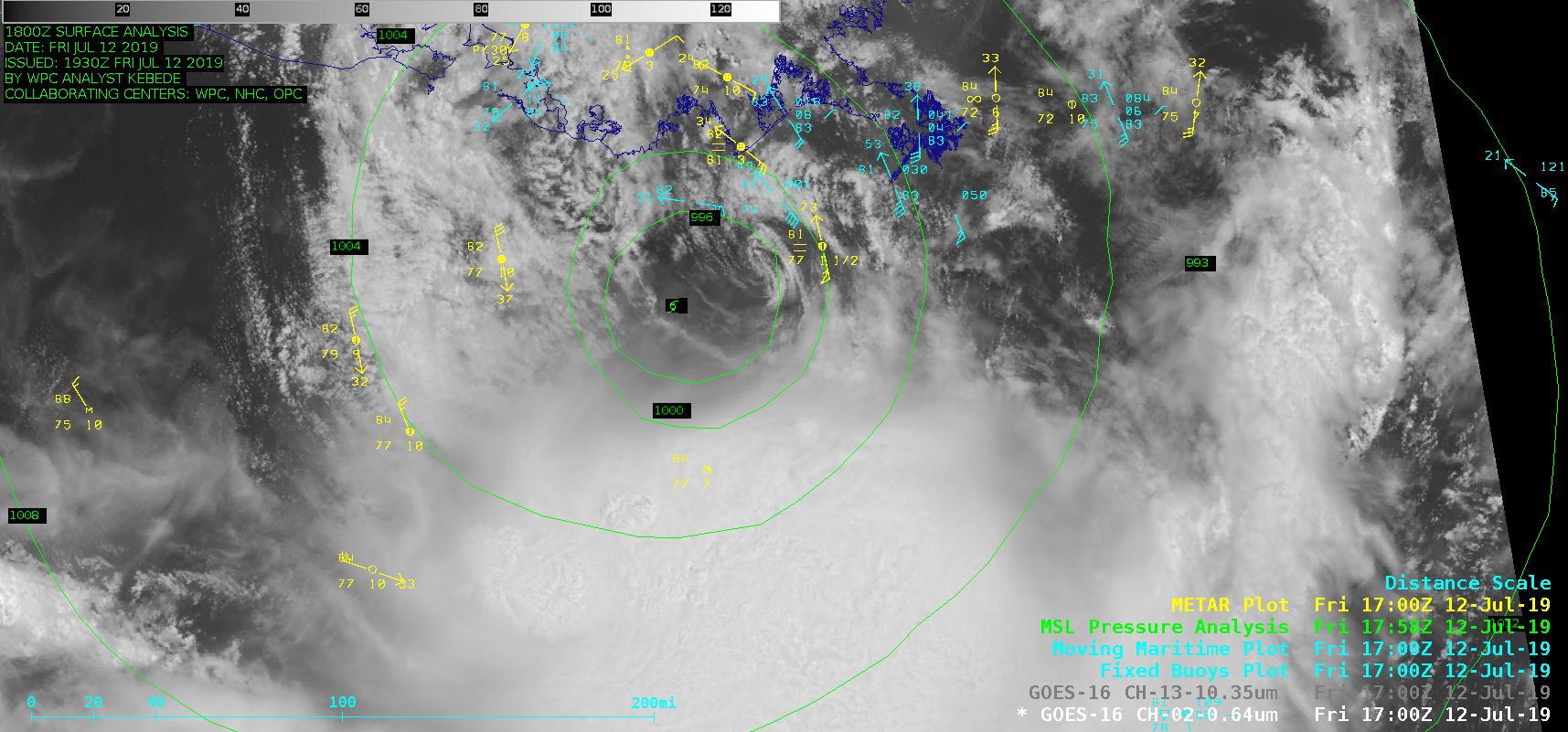
![GOES-16 "Red" Visible (0.64 µm) and "Clean" Infrared Window (10.35 µm) images, with plots of buoy and ship reports [click to play MP4 animation]](https://cimss.ssec.wisc.edu/satellite-blog/wp-content/uploads/sites/5/2019/07/barry_vis-20190711_150110.png)
GOES-16 “Red” Visible (0.64 µm) and “Clean” Infrared Window (10.35 µm) images, with plots of buoy and ship reports [click to play MP4 animation]
formed in the far northern Gulf of Mexico on
11 July 2019 — 1-minute
Mesoscale Domain Sector GOES-16
(GOES-East) “Red” Visible (
0.64 µm) and “Clean” Infrared Window (
10.35 µm) images
(above) displayed increasing convection associated with the tropical cyclone. The coldest cloud-top infrared brightness temperatures were -86ºC.
As was seen in an animation of GOES-16 Infrared imagery from the CIMSS Tropical Cyclones site (below), Barry was in an environment of low deep-layer wind shear — a factor that was favorable for further intensification.
![GOES-16 Infrared (11.2 µm) images, with contours of deep-layer wind shear [click to enlarge]](https://cimss.ssec.wisc.edu/satellite-blog/wp-content/uploads/sites/5/2019/07/190711_goes16_ir_shear_Barry_anim.gif)
GOES-16 Infrared (11.2 µm) images, with contours of deep-layer wind shear [click to enlarge]
===== 12 July Update =====
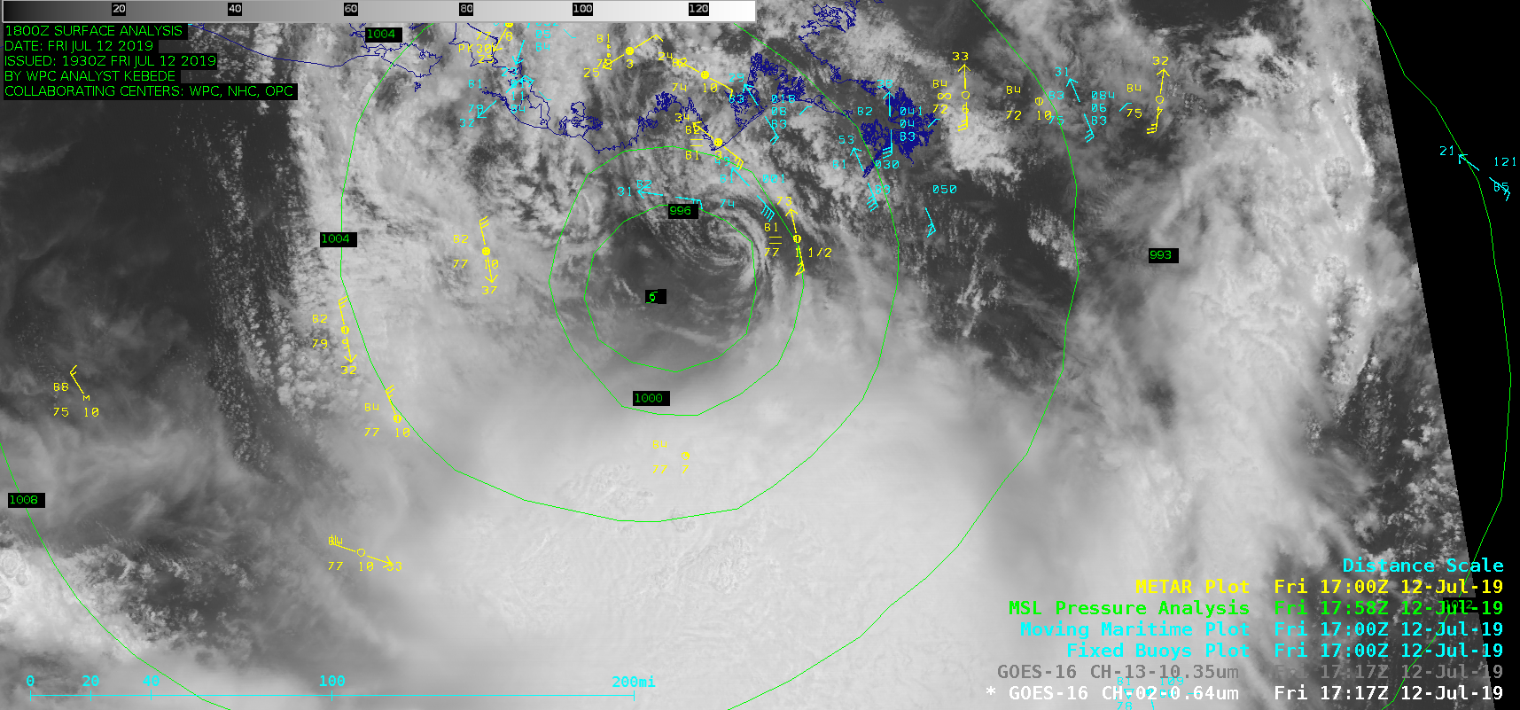
GOES-16 “Red” Visible (0.64 µm) images [click to play animation | MP4]
1-minute GOES-16 Visible images
(above) revealed a mesovortex that was rotating counter-clockwise around the low-level circulation center of Barry, which was approaching the coast of Louisiana on 12 July. Note that the METAR site located immediately east of the mesovortex around
17 UTC — KMDJ, Mississippi Canyon Oil Platform — had a wind gust of 73 knots or 84 mph around that time (and later had a wind gust to
90 mph at 2135 UTC or 4:35 PM CDT)
The corresponding GOES-16 Infrared images (below) showed that deep convection remained to the south of the center of Barry.
![GOES-16 "Clean" Infrared Window (10.35 µm) images [click to play animation | MP4]](https://cimss.ssec.wisc.edu/satellite-blog/wp-content/uploads/sites/5/2019/07/barry_ir-20190712_171710.png)
GOES-16 “Clean” Infrared Window (10.35 µm) images [click to play animation | MP4]
===== 17 July Update =====
![Aqua MODIS Sea Surface Temperature product [click to enlarge]](https://cimss.ssec.wisc.edu/satellite-blog/wp-content/uploads/sites/5/2019/07/modis_sst-20190709_073100.png)
Aqua MODIS Sea Surface Temperature product on 09 July [click to enlarge]
An Aqua MODIS Sea Surface Temperature image 2 days prior to the formation of Tropical Storm Barry
(above) showed SST values in the upper 80s to low 90s F
(darker shades of orange to red) in the northern Gulf of Mexico just south of Louisiana.
8 days later, a Terra MODIS SST image (below) revealed values predominantly in the lower to middle 80s F (green to yellow enhancement) — the slow movement of Barry as it eventually reached hurricane intensity just prior to landfall induced an upwelling of cooler sub-surface water over that area.
![Terra MODIS Sea Surface Temperature product on 17 July [click to enlarge]](https://cimss.ssec.wisc.edu/satellite-blog/wp-content/uploads/sites/5/2019/07/modis_sst-20190717_040600.png)
Terra MODIS Sea Surface Temperature product on 17 July [click to enlarge]
View only this post
Read Less
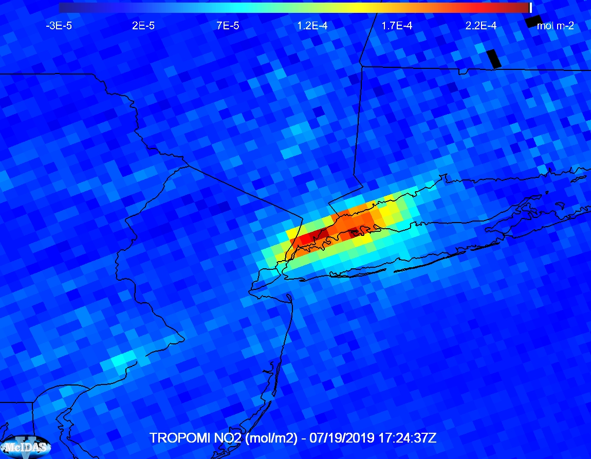
![TROPOMI NO2 concentration [click to enlarge]](https://cimss.ssec.wisc.edu/satellite-blog/wp-content/uploads/sites/5/2019/07/TROPOMI_NO2_NorthEast.jpg)
![TROPOMI NO2 concentration [click to enlarge]](https://cimss.ssec.wisc.edu/satellite-blog/wp-content/uploads/sites/5/2019/07/TROPOMI_NO2_NYC.jpg)
![Aqua MODIS Land Surface Temperature, with plots of daily maximum surface air temperatures [click to enlarge]](https://cimss.ssec.wisc.edu/satellite-blog/wp-content/uploads/sites/5/2019/07/190719_1737utc_aqua_modis_landSurfaceTemperature_dailyMaximimumAirTemperature_Northeast_US_anim.gif)

![GOES-16 "Clean" Infrared Window (10.35 µm) images [click to play animation | MP4]](https://cimss.ssec.wisc.edu/satellite-blog/wp-content/uploads/sites/5/2019/07/190712_goes16_infrared_Barry_anim.gif)
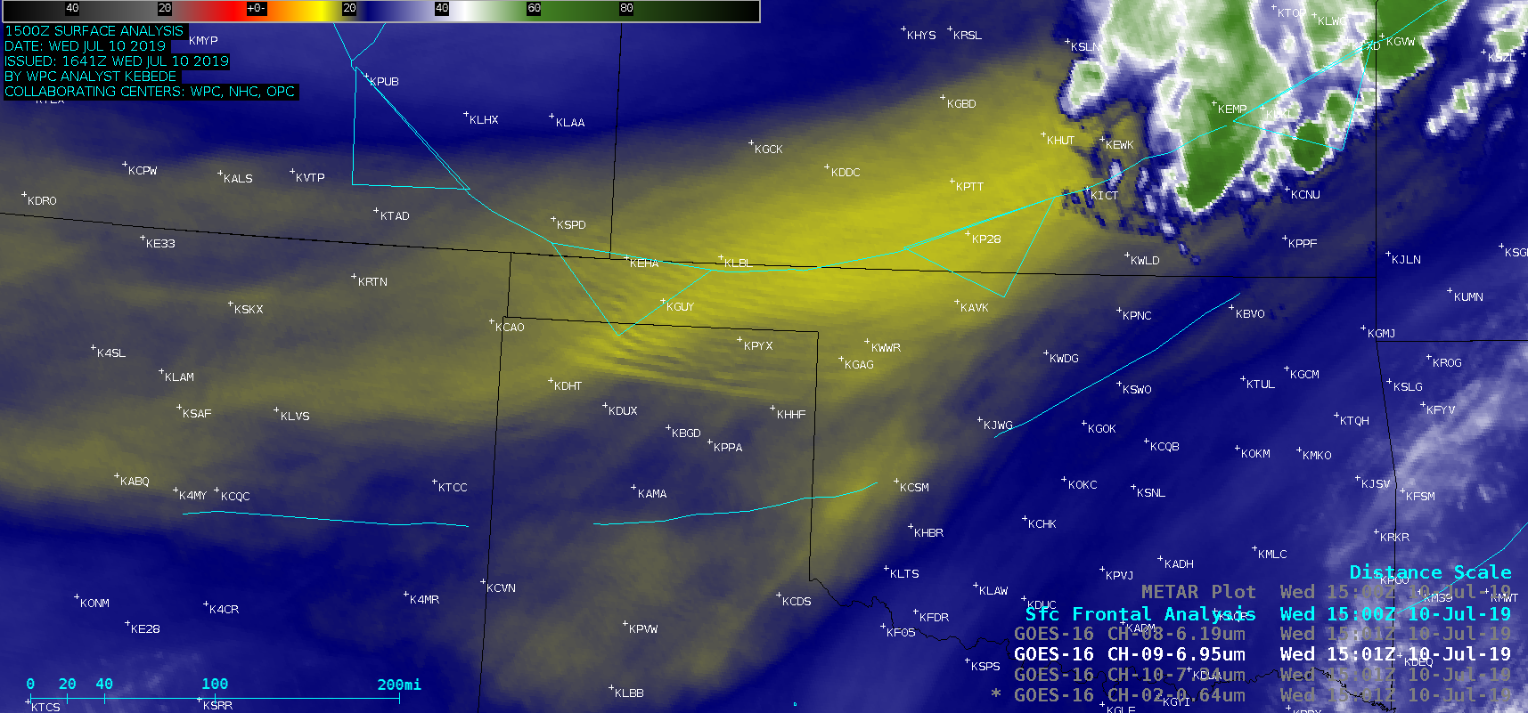
![GOES-17 Upper-level Water Vapor images, with pilot reports of turbulence [click to play animation | MP4]](https://cimss.ssec.wisc.edu/satellite-blog/wp-content/uploads/sites/5/2019/07/190711_goes17_waterVapor_band8_pireps_anim.gif)
![GOES-17 Mid-level Water Vapor (6.9 µm) images, with pilot reports of turbulence [click to play animation | MP4]](https://cimss.ssec.wisc.edu/satellite-blog/wp-content/uploads/sites/5/2019/07/190711_goes17_waterVapor_band9_pireps_anim.gif)

