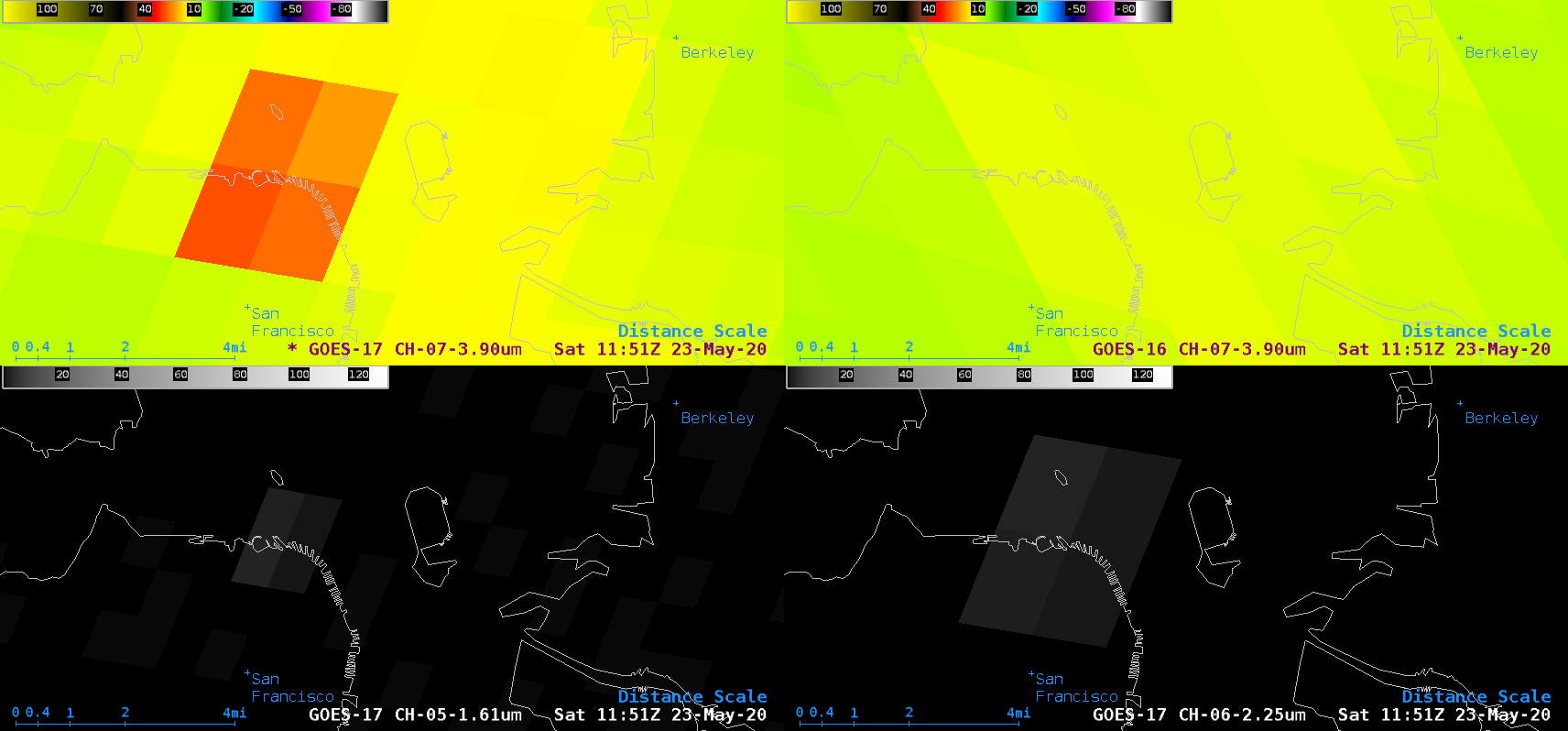
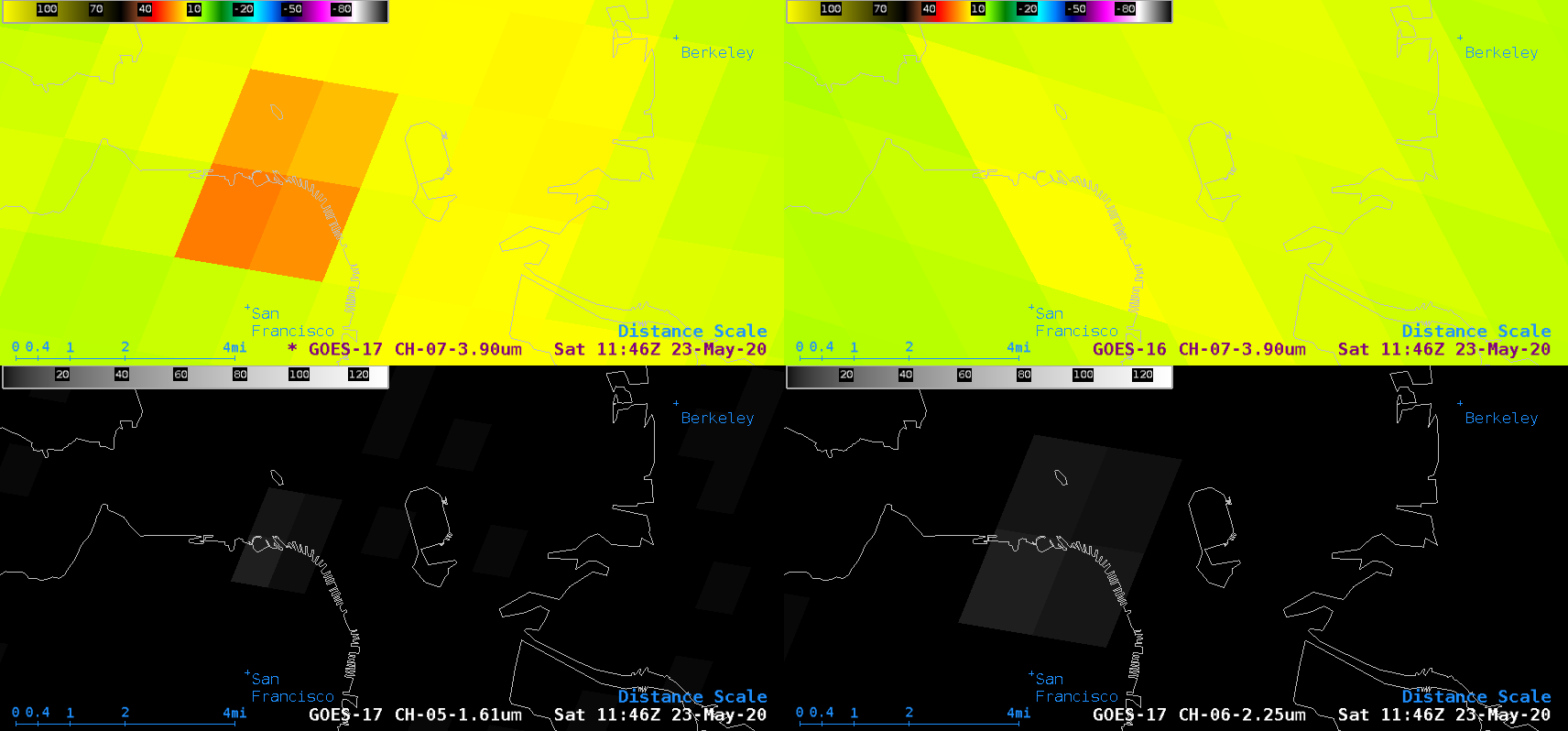
This website works best with a newer web browser such as Chrome, Firefox, Safari or Microsoft Edge. Internet Explorer is not supported by this website.

Using Polar2Grid software to create JPSS Imagery

Polar2Grid is Python-based software created at CIMSS/SSEC to process data from Polar Orbiting satellites into useful imagery (or into files that can be imported directly into the National Weather Service Advanced Weather Information Processing System (AWIPS) for display). (You can download it for a linux machine at this site.) This tutorial... Read More

NOAA-20 VIIRS Imagery (Image bands I01 (0.64 µm), I03 (1.61 µm) and I05 (11.45 µm)) at 23:25 UTC on 8 April 2019 (Click to enlarge)

Polar2Grid is Python-based software created at CIMSS/SSEC to process data from Polar Orbiting satellites into useful imagery (or into files that can be imported directly into the National Weather Service Advanced Weather Information Processing System (AWIPS) for display). (You can download it for a linux machine at this site.) This tutorial will describe where to find downloadable NOAA-20 (or Suomi-NPP) data, and how to create imagery. Thus, this blog post is similar to earlier blogs posts (here, and here) that described how to use Geo2Grid for Geostationary Satellites. Earlier blog posts showing Polar2Grid output are here and here.

There are data repositories associated with many direct broadcast antennas — but they are not always publically available. NOAA CLASS data is a reliable source for NOAA-20 and Suomi-NPP data. Typically data shows up there within six hours of its being sampled by the satellite. For a post-event analysis, this is a good data source. For near-real time investigation, it’s better to acquire data from a direct broadcast site. (Data from the Direct Broadcast antenna at CIMSS are available here.)

The first thing required at the NOAA CLASS site is to request the data that you want to access. There is a long drop-down menu (‘Please select a product to search’ is its original title) on the CLASS front page; use the drop down to select ‘JPSS Visible Infrared Imaging Radiometer Suite Sensor Data Record (VIIRS_SDR)’. This tells CLASS that you want VIIRS data from either Suomi NPP or NOAA-20. Click on the ‘Go’ button to the right of the menu bar. That takes you to a selection page.

It is necessary to log into the CLASS system. When you order data, an email is sent acknowledging the order, and a follow-on email once the data are available specifies how you can download it. The log-in tells CLASS where to send the emails.

Polar2Grid expects the data to be ‘de-aggregated’, so you must set User Preferences in NOAA CLASS to do this. Click on the ‘User Preferences’ link in the table on the left-hand side of the main NOAA CLASS Page (after you have logged in). The location is shown below in the toggle.

NOAA Class Front Page after logging in as a user. Note the ‘User Preferences’ Tab, circled in red.

Once you have entered the User Preference page, make certain that the ‘Package Geolocation with JPSS Data Products’ button is toggled to ‘No’. (Shown here) You also do want to De-aggregate JPSS Data Products. (That is, separate files for each band). In practice, this blogger finds it easier (that is, Polar2Grid complains less) if I make separate data requests at CLASS for each VIIRS band I want to view. (Update: ‘JPSS Companion Files to deliver with data’ should also be blank, as as shown at the link. This allows for one data request.)

Data requests require you to know something about the orbits of the satellites — so you can narrow down the amount of data you want. This handy website shows where all polar orbiters have been flying. Follow the links to the specific satellite and location; for example, if we’re interested in NOAA-20 orbits over Hawai’i on April 8 2019, this map shows them. The map suggests requesting NOAA-20 from 23:20 to 23:30 on 8 April 2019 will give a good view of the islands.

The data we will request are I01, I03 and I05 (0.64 µm, 1.61 µm and 11.45 µm, respectively). In addition to requesting the Sensor Data Records, it is also necessary to request, near the bottom of the page, the ‘VIIRS Image Bands SDR Ellipsoid Terrain Corrected Geolocation (GITCO) (public)’. These geolocation files are used by Polar2Grid to navigate the imagery.

After submitting the data request, and waiting a period of time (sometimes as short as two or three minutes), you will receive an email telling you exactly where the data sits, and how to access it. It will look something like this. Download the data into a directory, and you’re ready to have Polar2Grid create imagery for you. The directory for I05 (I will put data for each band in a separate directory) should include files named like this:

GIMGO_j01_d20190408_t2320306_e2321551_b07188_c20190409223158545413_noac_ops.h5
GITCO_j01_d20190408_t2320306_e2321551_b07188_c20190409223155222712_noac_ops.h5
SVI03_j01_d20190408_t2320306_e2321551_b07188_c20190409223158545413_noac_ops.h5

‘GIMGO’ and ‘GITCO’ refer to geolocation data; even though you only requested GITCO fields, CLASS will give both. That’s okay. SVI01, SVI03 and SVI05 hold data from bands I01, I03 and I05, respectively. The ‘j01’ tag signifies data from NOAA-20, or JPSS-1. For the 20-minute request I made for each band, I received 8 of each type of file.

The Polar2Grid command that creates imagery is this one:

polar2grid.sh viirs_sdr gtiff -p i03 -f /home/scottl/Polar2Grid/data/viirs/I03/

The polar2grid.sh shell script is within the bin directory of the Polar2Grid software that emerges after you g-unzip and untar the file from the Polar2Grid download site. The command results in a .tif file with highest-resolution grey-scaled imagery. The image below (converted from .tif to .png) shows the scene. It’s quite large: 6876×7616 pixels!

NOAA-20 Imagery (I-3, 1.61 µm) from 23:20 to 23:30 on 8 April 2019 (Click to enlarge)

It’s useful to add maps to the imagery, and that is done in Polar2Grid after the .tif file has been created by using ‘add_coastlines.sh’, also in the bin directory. The command can add coastlines (–add-coastlines), borders (–add-borders), rivers (–add-rivers) and lat/lon lines (–add-grid). Lat/Lon lines can also be labeled. When maps are added to the .tif file, the image is also saved as a .png file so the original scene is not overwritten. You can use the -o flag to rename the new file. The command I used is shown below.

add_coastlines.sh –add-coastlines j01_viirs_i03_20190408_231906_wgs84_fit.tif –coastlines-resolution=f –coastlines-level=6 –coastlines-outline=’magenta’ -o j01_I03_20190408_231906.png

After adding maps to all three files created, I used ImageMagick to crop the large fields to something more manageable in size (convert -crop 1520×900+2112+2409 +repage -quality 100 j01_I05_20190408_231906.png j01_I05_20190408_231906.gif, for example), and added annotation to the imagery:

convert -font helvetica -fill yellow -pointsize 36 -draw “text 70,70 ‘NOAA-20 VIIRS Image Band I01 (0.64 µm) 23:25 UTC 8 April 2019′” j01_I01_20190408_231906.gif j01_I01_20190408_231906.annot.gif

The animation at the top of this blog post shows all three images (I01, I03 and I05) sequentially.

Final note: Infrared imagery by default is not color-enhanced, and built-in enhancements are not (yet) available. Polar2Grid does support creation of colortables, however. That will be the subject of a future blog post.

View only this post Read Less

Fires in the Plains

GOES-16 (GOES-East) Shortwave Infrared (3.9 µm) images and the corresponding GOES-16 Fire Temperature product (above) showed the thermal signatures of widespread fires across the Great Plains (primarily in the Flint Hills of Kansas and Oklahoma) on 08 April 2019. Although fairly small and often relatively brief, some of these fires become quite hot —... Read More

GOES-16 Shortwave Infrared (3.9 µm) and Fire Temperature product [click to play animation | MP4]

GOES-16 Shortwave Infrared (3.9 µm) and Fire Temperature product [click to play animation | MP4]

GOES-16 (GOES-East) Shortwave Infrared (3.9 µm) images and the corresponding GOES-16 Fire Temperature product (above) showed the thermal signatures of widespread fires across the Great Plains (primarily in the Flint Hills of Kansas and Oklahoma) on 08 April 2019. Although fairly small and often relatively brief, some of these fires become quite hot — exhibiting Fire Temperature values as high as 2762 K (or 4512ºF) southwest of Cottonwood, Kansas at 2011 UTC. These fires were typical Springtime prescribed burns and agricultural fields being cleared for planting.

One fire southwest of Salina, Kansas began to exhibit a prominent 3.9 µm thermal anomaly after 22 UTC, attaining a peak infrared brightness temperature of 95.6ºC (or 204ºF); a closer view of that fire is shown using GOES-16 Shortwave Infrared images along with Fire Temperature, Fire Area and Fire Power products (below). Note that during much of the time (for example, at 2221 UTC) there were no Fire Temperature, Fire Area or Fire Power values processed for the hottest 3.9 µm fire pixel — this is because the fire was producing a thick smoke plume, and the smoke-filled (on Visible imagery) hot pixel was flagged by the GOES Fire Detection and Characterization Algorithm (FDCA) Cloud Mask as a “cloudy pixel”. Beginning in May 2019, an updated algorithm will begin to produce the Fire Power parameter for all types of fire pixel (Processed fire, Saturated fire, Cloud-contaminated fire, and High/Medium/Low-probability fires), but the Fire Temperature and Fire Size parameters will only be available for the Processed fire category.

GOES-16 Shortwave Infrared (3.9 µm, upper left), Fire Temperature (upper right), Fire Area (lower left) and Fire Power (lower right) [click to play animation | MP4]

GOES-16 Shortwave Infrared (3.9 µm, upper left), Fire Temperature (upper right), Fire Area (lower left) and Fire Power (lower right) [click to play animation | MP4]

A sequence of MODIS and VIIRS Shortwave Infrared (3.7 µm) images from the Aqua, Suomi NPP and NOAA-20 satellites (below) showed a more detailed view of the fire thermal signatures (black to yellow to red enhancement) during the 1.5 hours between 1822 and 2001 UTC.

Sequence of MODIS and VIIRS Shortwave Infrared (3.7 µm) images from 1822-2001 UTC [click to enlarge]

Sequence of MODIS and VIIRS Shortwave Infrared (3.7 µm) images from 1822-2001 UTC [click to enlarge]

Most of the small fires did not produce particularly large smoke plumes, but the density of the fires led to a rather large pall of smoke over the region as seen in GOES-16 “Red” Visible (0.64 µm) images (below).
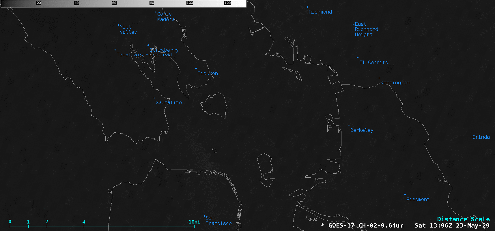
 Note the smoke plume emanating from the fire southwest of Salina, Kansas (as previously discussed). Most of the smoke was dispersed above the boundary layer — but the surface visibility was reduced by smoke at sites such as Coffeyville, Chanute and Eureka in southeastern Kansas and Bartlesville in northeastern Oklahoma.

GOES-16 "Red" Visible (0.64 µm) images [click to play animation | MP4]

GOES-16 “Red” Visible (0.64 µm) images [click to play animation | MP4]

===== 09 April Update ====

NOAA-20 VIIRS Day/Night Band (0.7 µm) and Shortwave Infrared (3.74 µm) images [click to enlarge]

NOAA-20 VIIRS Day/Night Band (0.7 µm) and Shortwave Infrared (3.74 µm) images [click to enlarge]

As some of the larger fires in southern Kansas continued burning into the night, their thermal signature could be seen in NOAA-20 VIIRS Shortwave Infrared (3.74 µm) image (darker gray to black pixels), along with their bright glow in the corresponding VIIRS Day/Night Band (0.7 µm) image at 0818 UTC or 3:18 am CDT (above). Note: the NOAA-20 images are incorrectly labeled as Suomi NPP.

View only this post Read Less

Large hail in Texas

1-minute Mesoscale Domain Sector GOES-16 (GOES-East) “Red” Visible (0.64 µm) images with plots of GLM Groups (above) showed a large and electrically-active Mesoscale Convective System (MCS) which produced hail up to 4.5 inches in diameter (SPC storm reports) in eastern Texas on 06 Aprill 2019. These severe thunderstorms intensified generally along and north of a quasi-stationary frontal... Read More

GOES-16

GOES-16 “Red” Visible (0.64 µm) images, with GLM Groups plotted in cyan and SPC storm reports plotted in red [click to play animation | MP4]

1-minute Mesoscale Domain Sector GOES-16 (GOES-East) “Red” Visible (0.64 µm) images with plots of GLM Groups (above) showed a large and electrically-active Mesoscale Convective System (MCS) which produced hail up to 4.5 inches in diameter (SPC storm reports) in eastern Texas on 06 Aprill 2019. These severe thunderstorms intensified generally along and north of a quasi-stationary frontal boundary (surface analyses).

The corresponding GOES-16 “Clean” Infrared Window (10.3 µm) images (below) showed that cloud-top infrared brightness temperatures associated with the strongest overshooting tops were around -70ºC (dark black enhancement). Earlier that afternoon, a higher spatial resolution Suomi NPP VIIRS Infrared Window (11.45 µm) image at 1950 UTC showed brightness temperatures as cold as -77ºC just northeast of where 2.0-inch diameter hail was reported at Marquez — located approximately midway between station identifiers KLHB and KPSN — at 2015 UTC. Assuming the 00 UTC Lake Charles sounding was representative of the air mass these storms were developing in, the -77ºC temperature would be at an altitude over 1 km higher than the Most Unstable parcel’s Equilibrium Level.

GOES-16 "Clean" Infrared Window (10.3 µm) images, with GLM Groups plotted in beige and SPC storm reports plotted in cyan [click to play animation | MP4]

GOES-16 “Clean” Infrared Window (10.3 µm) images, with GLM Groups plotted in beige and SPC storm reports plotted in cyan [click to play animation | MP4]

With better cloud-top shadow contrast, GOES-16 Near-Infrared “Snow/Ice” (1.61 µm) images (below) were helpful to locate the presence of Above-Anvil Cirrus Plume (AACP) features with the 2 strongest cells — and a comparison with 10.3 µm Infrared images indicated slightly warmer brightness temperatures with these AACPs (for example, at 2244 UTC and  0005 UTC).

GOES-16 Near-Infrared "Snow/Ice" (1.61 µm) images, with SPC storm reports plotted in red [click to play animation | MP4]

GOES-16 Near-Infrared “Snow/Ice” (1.61 µm) images, with SPC storm reports plotted in red [click to play animation | MP4]

GOES-16 All Sky Total Precipitable Water (TPW) and Convective Available Potential Energy (CAPE) products (below) showed the areal coverage and trends in moisture and instability across the region on that day.

GOES-16 All Sky Total Precipitable Water (TPW) images [click to play animation]

GOES-16 All Sky Total Precipitable Water (TPW) product [click to play animation]


GOES-16 All Sky Convective Available Potential Energy (CAPE) product [click to play animation]

GOES-16 All Sky Convective Available Potential Energy (CAPE) product [click to play animation]

View only this post Read Less

Wildfires on the Korean Peninsula

2.5-minute rapid scan JMA Himawari-8 Shortwave Infrared (3.9 µm) images (above) showed numerous thermal anomaly (or “hot spot”, darker red to black pixels) signatures of wildfires across southeastern North Korea and northeastern South Korea on 04 April 2019 (media story). The fires were fanned by strong west-southwest winds in the wake... Read More

JMA Himawari-8 Shortwave Infrared (3.9 µm) images, with plots of surface reports (metric units) [click to play animation | MP4]

JMA Himawari-8 Shortwave Infrared (3.9 µm) images, with hourly plots of surface reports in metric units [click to play animation | MP4]

2.5-minute rapid scan JMA Himawari-8 Shortwave Infrared (3.9 µm) images (above) showed numerous thermal anomaly (or “hot spot”, darker red to black pixels) signatures of wildfires across southeastern North Korea and northeastern South Korea on 04 April 2019 (media story). The fires were fanned by strong west-southwest winds in the wake of a cold frontal passage associated with an anomalously-deep midlatitude cyclone moving across far northeastern China (surface analyses); winds gusted to 53 knots at Yangyang International Airport (station identifier RKNY) to the south of Sokcho at 09 UTC (below). Standing wave clouds — forming in response to the strong westerly winds — were seen downwind of the mountainous terrain of the eastern Korean Peninsula from 1030-1930 UTC.

Time series of surface weather data at Yangyang, South Korea [click to enlarge]

Time series of surface weather data at Yangyang, South Korea [click to enlarge]

Comparisons of VIIRS Day/Night Band (0.7 µm), Near-infrared (1.61 µm and 2.25 µm), Shortwave Infrared (3.75 µm and 4.05 µm) and Infrared Window (11.45 µm) images from NOAA-20 at 1649 UTC and Suomi NPP at 1739 UTC are shown below (courtesy of William Straka, CIMSS). A subtle thermal signature of the largest fires — located between Gangneug and Donghae, and also near Sokcho — was even apparent as darker pixels on the Infrared Window (I-Band 5, 11.45 µm) images. On the Day/Night Band images, note the striking lack of city lights in the southeastern portion of North Korea in these nighttime scenes.

NOAA-20 VIIRS Day/Night Band (0.7 µm), Near-infrared (1.61 µm and 2.24 µm), Shortwave Infrared (3.75 µm and 4.05 µm) and Infrared Window (11.45 µm) images [click to enlarge]

NOAA-20 VIIRS Day/Night Band (0.7 µm), Near-infrared (1.61 µm and 2.25 µm), Shortwave Infrared (3.75 µm and 4.05 µm) and Infrared Window (11.45 µm) images at 1649 UTC [click to enlarge]

Suomi NPP VIIRS Day/Night Band (0.7 µm), Near-infrared (1.61 µm and 2.24 µm), Shortwave Infrared (3.75 µm and 4.05 µm) and Infrared Window (11.45 µm) images [click to enlarge]

Suomi NPP VIIRS Day/Night Band (0.7 µm), Near-infrared (1.61 µm and 2.25 µm), Shortwave Infrared (3.75 µm and 4.05 µm) and Infrared Window (11.45 µm) images at 1739 UTC [click to enlarge]

Thermal signatures of the fires were also captured by KMA COMS-1 Shortwave Infrared (3.9 µm) imagery (below), but not as well as with Himawari-8 given the inferior spatial resolution (4 km, vs 2 km for Himawari-8) and image frequency (15 minutes, vs 2.5 minutes with the Himawari-8 Japan Sector).

KMA COMS-1 Shortwave Infrared (3.9 µm) images, with hourly plots of surface reports in metric units [click to play animation | MP4]

KMA COMS-1 Shortwave Infrared (3.9 µm) images, with hourly plots of surface reports in metric units [click to play animation | MP4]

View only this post Read Less