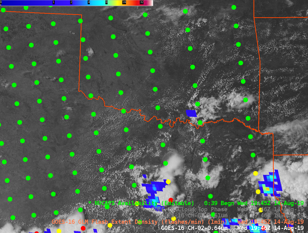
GOES-16 Visible Imagery, above (Click to animate), shows shower/thundershower development over eastern Oklahoma moving into Arkansas. At the end of the animation, 1946 UTC, NUCAPS Sounding profiles from 1926 UTC are shown, and they’re shown below too.The time 1946 UTC is about the earliest you could hope to have NUCAPS... Read More
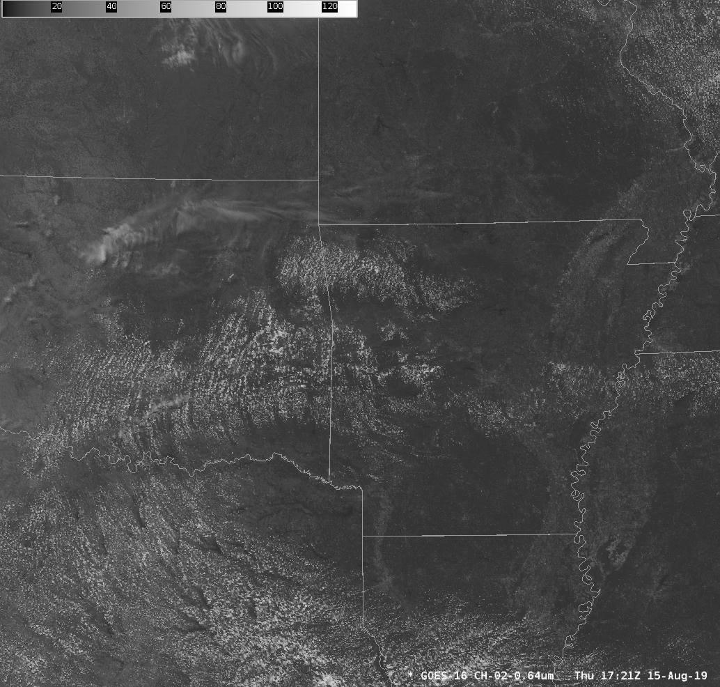
GOES-16 Visible (Band 2, 0.64 µm) Imagery, 1721 – 1946 UTC on 15 August 2019. NUCAPS Sounding Points — from 1926 UTC — are present over the image at 1946 UTC (Click to animate)
GOES-16 Visible Imagery, above (Click to animate), shows shower/thundershower development over eastern Oklahoma moving into Arkansas. At the end of the animation, 1946 UTC, NUCAPS Sounding profiles from 1926 UTC are shown, and they’re shown below too.

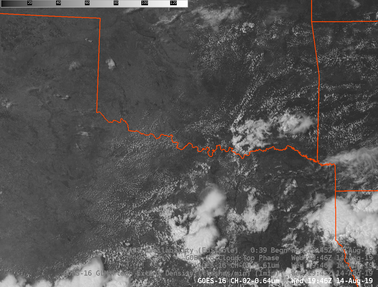
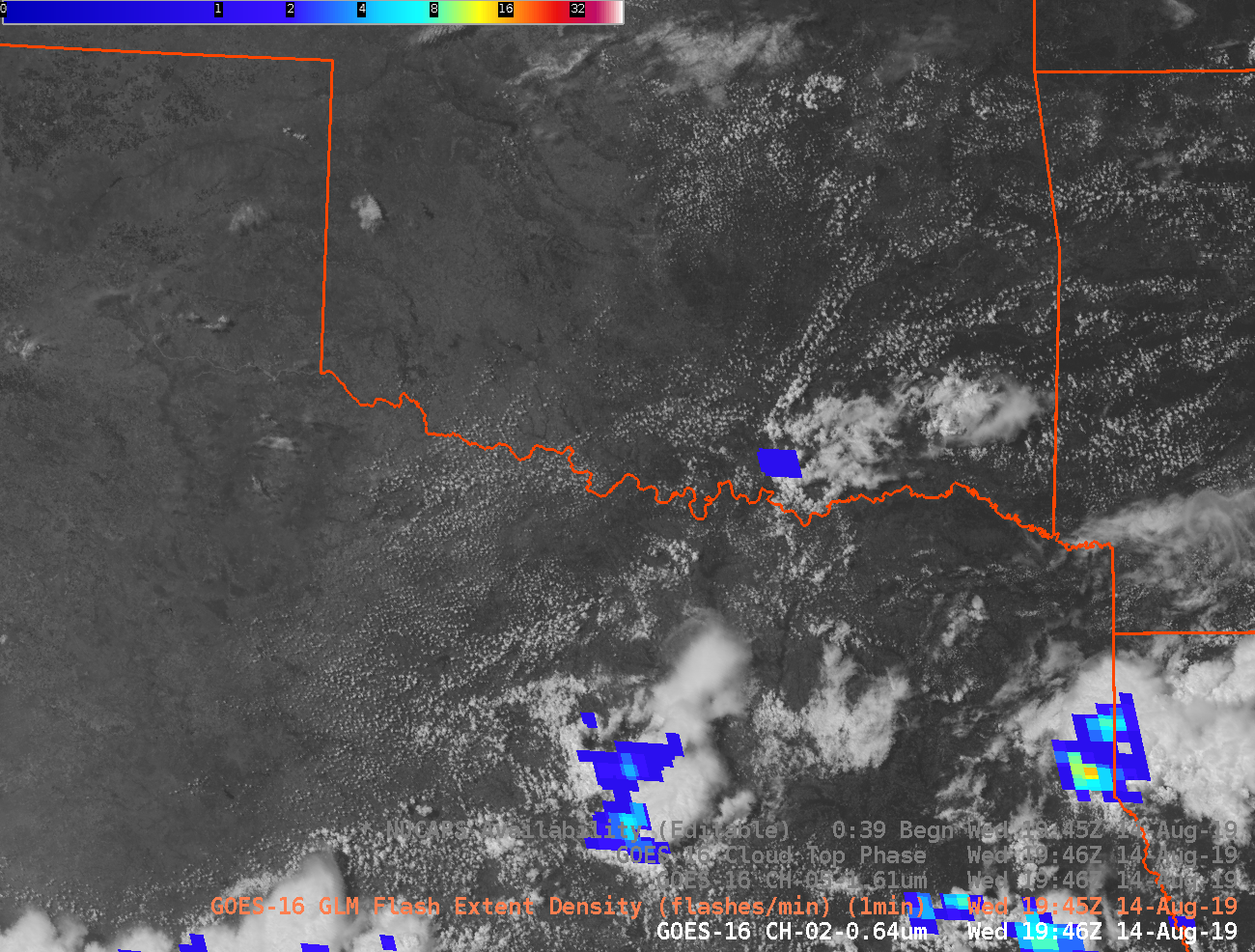
GOES-16 Visible (Band 2, 0.64 µm) Imagery, 1946 UTC on 15 August 2019. (Click to enlarge)
The time 1946 UTC is about the earliest you could hope to have NUCAPS profiles in an AWIPS system — and only if you had access to a Direct Broadcast antenna. The more conventional method of data delivery, the SBN, means NUCAPS will be available about an hour after they are taken, so by 2036 UTC. The visible imagery at 2036 UTC is shown below.
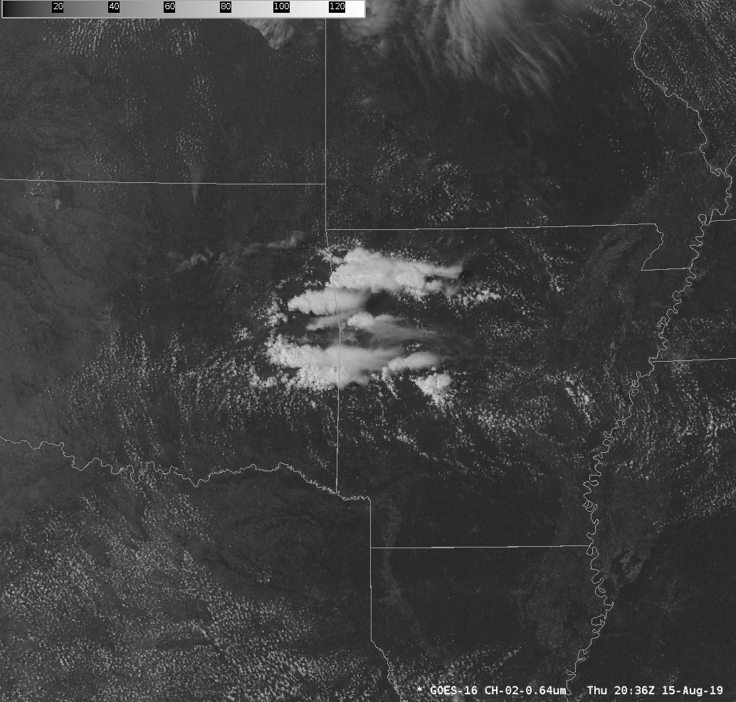
GOES-16 Visible (Band 2, 0.64 µm) Imagery, 1946 UTC on 15 August 2019. (Click to enlarge)
At 2036 UTC, which time is about when in the forecast office the NUCAPS soundings would become available, would you expect the convection in western Arkansas to move southward, or eastward, based solely on Satellite imagery? How could you use NUCAPS profiles to gain confidence in this prediction? Visible imagery alone suggests a moisture boundary; the southern quarter of Arkansas shows markedly less cumulus cloudiness. The animation shows motion mostly to the east, with higher clouds moving more west-northwesterly. The GOES-16 Baseline Total Precipitable Water product, below, shows a maximum in TPW over central Arkansas, with values around 1.5″; values are around 1.3″ in southern Arkansas, and around 1.2-1.3″ in northwest Arkansas. A corridor of moisture is indicated.

GOES-16 Baseline Level 2 Total Precipitable Water at 1946 UTC; Visible imagery is shown in cloudy regions. (Click to enlarge)
Baseline Total Precipitable Water, above, part of a suite of products that emerge from Legacy Profiles, is heavily constrained by model fields, however; the image above could simply show the GFS solution. In contrast, NUCAPS observations are almost wholly independent of models. What do NUCAPS profiles show? The animation below steps through vertical profiles east and south of the developing convection.
NUCAPS profiles from the ~1900 UTC overpass at points plotted over the 1946 UTC GOES-16 Band 2 Visible (0.64 µm) image (Click to enlarge)
AWIPS will soon (planned for shortly after Labor Day at the time of this post) include horizontal fields of information derived from NUCAPS vertical profiles. The images below show values computed within the NSharp AWIPS software for a variety of fields: Total Precipitable Water, MU Lifted Index, MU CAPE, MU CINH. All fields suggest that convection more likely to build eastward than to expand southward.
NUCAPS Sounding Points and derived quantities, as indicated, at 1926 UTC 15 August 2019; NUCAPS data are plotted over the 1946 UTC GOES-16 ABI Band 2 Visible 0.64 µm image. (Click to enlarge)
Convection did not move southward; motion and development was to the east. The timing of NUCAPS profiles means that they give a good estimate of atmospheric thermodynamics in mid-afternoon, a key time for assessing convective development.
GOES-16 Visible (Band 2, 0.64 µm) Imagery, 1721 UTC on 15 August 2019 to 0001 UTC on 16 August 2019 (Click to animate).
View only this post
Read Less


![Time series of surface reports from Seward, Alaska [click to enlarge]](https://cimss.ssec.wisc.edu/satellite-blog/wp-content/uploads/sites/5/2019/08/190817_PAWD_SFCMG.GIF)
![Seward Airport webcam image at 2358 UTC [click to enlarge]](https://cimss.ssec.wisc.edu/satellite-blog/wp-content/uploads/sites/5/2019/08/190817_2358utc_Seward_airport_webcam.png)
![Air Quality Index at Copper Landing and Seward [click to enlarge]](https://cimss.ssec.wisc.edu/satellite-blog/wp-content/uploads/sites/5/2019/08/190817_Seward_AK_airQalityIndex.png)
![VIIRS True Color RGB images from NOAA-20 and Suomi NPP [click to enlarge]](https://cimss.ssec.wisc.edu/satellite-blog/wp-content/uploads/sites/5/2019/08/190817_noaa20_suomiNPP_viirs_trueColor_SwanLakeFire_AK_anim.gif)


