GOES-16 (GOES-East) “Red” Visible (0.64 µm) images (above) revealed the formation of a mesovortex in northern Lake Superior on 28 December 2020. Mid-lake convergence — as depicted by RAP40 model surface winds — contributed to the development of this feature.ASCAT surface scatterometer winds from Metop-A at 1537 UTC (below) provided a... Read More
![GOES-16 “Red” Visible (0.64 µm) images [click to play animation | MP4]](https://cimss.ssec.wisc.edu/satellite-blog/images/2020/12/lsup_mesovort-20201228_180118.png)
GOES-16 “Red” Visible (0.64 µm) images [click to play animation | MP4]
GOES-16
(GOES-East) “Red” Visible (
0.64 µm) images
(above) revealed the formation of a mesovortex in northern Lake Superior on 28 December 2020. Mid-lake convergence — as depicted by RAP40 model surface winds — contributed to the development of this feature.
ASCAT surface scatterometer winds from Metop-A at 1537 UTC (below) provided a good view of the cyclonic flow of the mesovortex in its early stages, before it became organized enough to become obvious on satellite imagery.
![GOES-16 Visible mage, with an overlay of Metop ASCAT surface scatterometer winds [click to enlarge]](https://cimss.ssec.wisc.edu/satellite-blog/images/2020/12/201218_1536utc_goes16_metop_acsat_Lake_Superior_mesovortex_anim.gif)
GOES-16 Visible mage, with and without an overlay of Metop ASCAT surface scatterometer winds [click to enlarge]
A toggle between ASCAT winds from Metop-A and Metop-B (
source) is shown below.
![ASCAT winds from Metop-A and Metop-B [click to enlarge]](https://cimss.ssec.wisc.edu/satellite-blog/images/2020/12/201228_metopA_metopB_ascat_Lake_Superior_mesovortex_anim.gif)
ASCAT winds from Metop-A and Metop-B [click to enlarge]
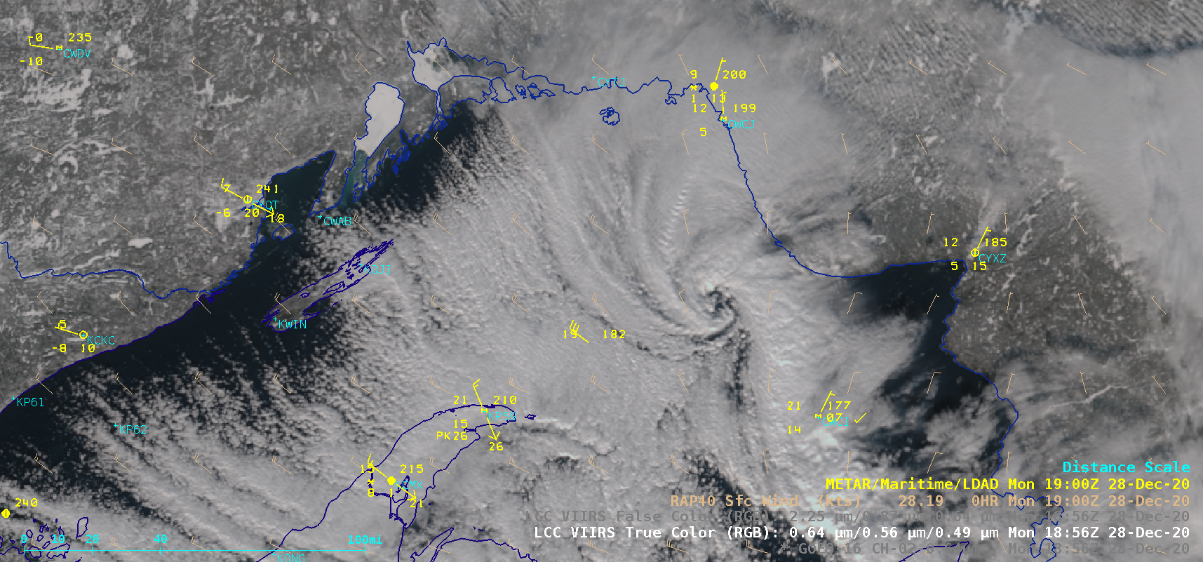
VIIRS True Color and False Color RGB images from Suomi NPP and NOAA-20
(below) showed a higher resolution view of the mesovortex; the shades of cyan in the False Color images suggested that the tops of some of the cloud bands were becoming glaciated.
![VIIRS True Color and False Color RGB images from Suomi NPP and NOAA-20 [click to enlarge]](https://cimss.ssec.wisc.edu/satellite-blog/images/2020/12/201228_viirs_trueColorRGB_falseColorRGB_Lake_Superior_mesovortex_anim.gif)
VIIRS True Color and False Color RGB images from Suomi NPP and NOAA-20 [click to enlarge]
False color images from VIIRS as shown above combine bands M11, I2 and I1: 2.25 µm, 0.865 µm and 0.64 µm. Inclusion of the near-IR channel at 2.25 µm causes a color change – less red (blue and green make cyan) – in regions where ice crystals exist, because ice crystals absorb, rather than reflect, solar energy at that wavelength. A similar occurrence happens at 1.61 µm wavelengths.
Accordingly, the Day Cloud Phase Distinction RGB, shown below, highlights ice crystals in clouds (they are yellow or orange because there is less green in the RGB where ice crystals are present; before sunrise, and after sunset, the RGB is only red: green and blue contributions depend on solar reflectance). Solar reflectance is small at all wavelengths at this time of year over Lake Superior, but a definite color difference in the clouds of the vortex is apparent. Snow showers/squalls are more likely where the Day Cloud Phase Distinction RGB suggests ice crystals in the clouds, as shown in this blog post (and this one!).
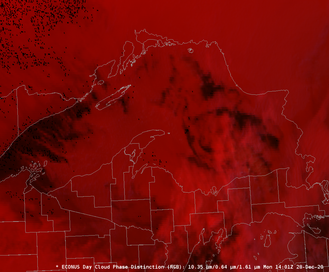
Day Cloud Phase Distinction RGB, 1401 UTC – 2131 UTC, 28 December 2020 (Click to animate)
Mesoscale vortices over warm lakes owe their existence to sensible and latent heat fluxes from the (relatively) warm water into the colder atmosphere aloft. (Click here for a presentation of such an event over southern Lake Michigan). When the vortex moved over Ontario and lost the lake fluxes, it dissipated. Visible imagery from the morning of 29 December 2020, below, showed no circulation.
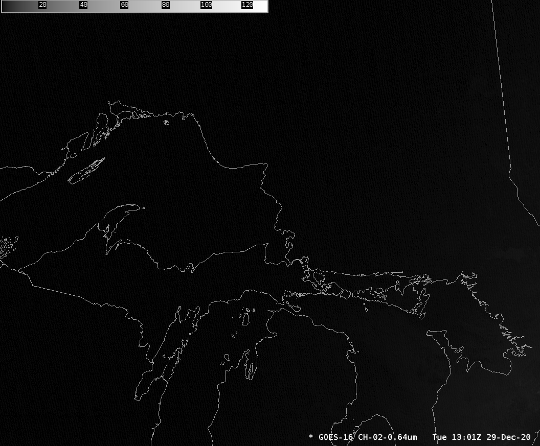
GOES-16 Visible Imagery (0.64 µm), 1301 – 1531 UTC on 29 December 2020 (Click to animate)
View only this post
Read Less

![GOES-17 Air Mass RGB and Mid-level Water Vapor (6.9 µm) images [click to play animation | MP4]](https://cimss.ssec.wisc.edu/satellite-blog/images/2020/12/201231_goes17_airMassRGB_waterVapor_AK_low_anim.gif)
![GOES-17 Mid-level Water Vapor (6.9 µm) image at 0910 UTC, with plots of Metop ASCAT surface scatterometer winds [click to enlarge]](https://cimss.ssec.wisc.edu/satellite-blog/images/2020/12/ak_ascat_wv-20201231_091032.png)
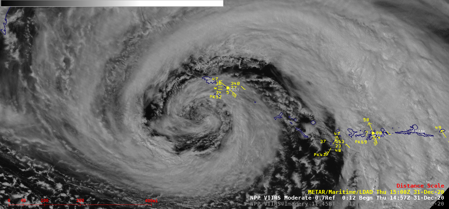
![Suomi NPP VIIRS Infrared Window (11.45 µm) and Day/Night Band (0.7 µm) images [click to enlarge]](https://cimss.ssec.wisc.edu/satellite-blog/images/2020/12/201231_1457utc_suomiNPP_viirs_infraredWindow_dayNightBand_AK_low_anim.gif)
![Suomi NPP VIIRS Infrared Window (11.45 µm) and Day/Night Band (0.7 µm) images [click to enlarge]](https://cimss.ssec.wisc.edu/satellite-blog/images/2020/12/210101_0053utc_suomiNPP_viirs_infraredWindow_dayNightBand_AK_low_anim.gif)
![GOES-17 Mid-level Water Vapor (6.9 µm) images, with contours of PV1.5 pressure [click to play animation | MP4]](https://cimss.ssec.wisc.edu/satellite-blog/images/2020/12/201231_goes17_waterVapor_pv1.5pressure_AK_low_anim.gif)
![Plot of surface report data from Shemya [click to enlarge]](https://cimss.ssec.wisc.edu/satellite-blog/images/2020/12/201231_PASY_SFCMG.GIF)
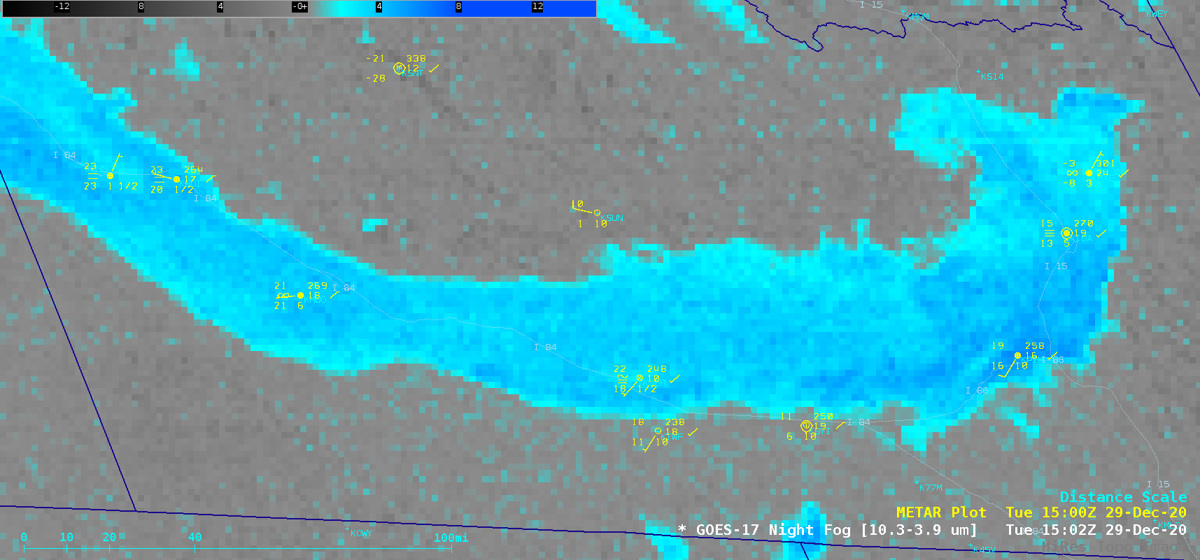
![GOES-17 Night Fog BTD and “Red” Visible (0.64 µm) [click to play animation | MP4]](https://cimss.ssec.wisc.edu/satellite-blog/images/2020/12/201229_goes17_nightFogBTD_visible_Idaho_fog_anim.gif)
![Suomi NPP VIIRS Day/Night Band (0.7 µm) image [click to enlarge]](https://cimss.ssec.wisc.edu/satellite-blog/images/2020/12/id_viirs_dnb-20201229_085601.png)
![GOES-16 “Red” Visible (0.64 µm) images [click to play animation | MP4]](https://cimss.ssec.wisc.edu/satellite-blog/images/2020/12/201228_goes16_visible_Lake_Superior_mesovortex_anim.gif)

