Showers developed over southern Wisconsin late in the day on 12 June 2020. What satellite products could be used to anticipate where the showers would develop? The animation of visible and radar, above, shows that the storms initiated near a boundary (mostly stationary) that separated Lake Michigan-influenced air with less... Read More

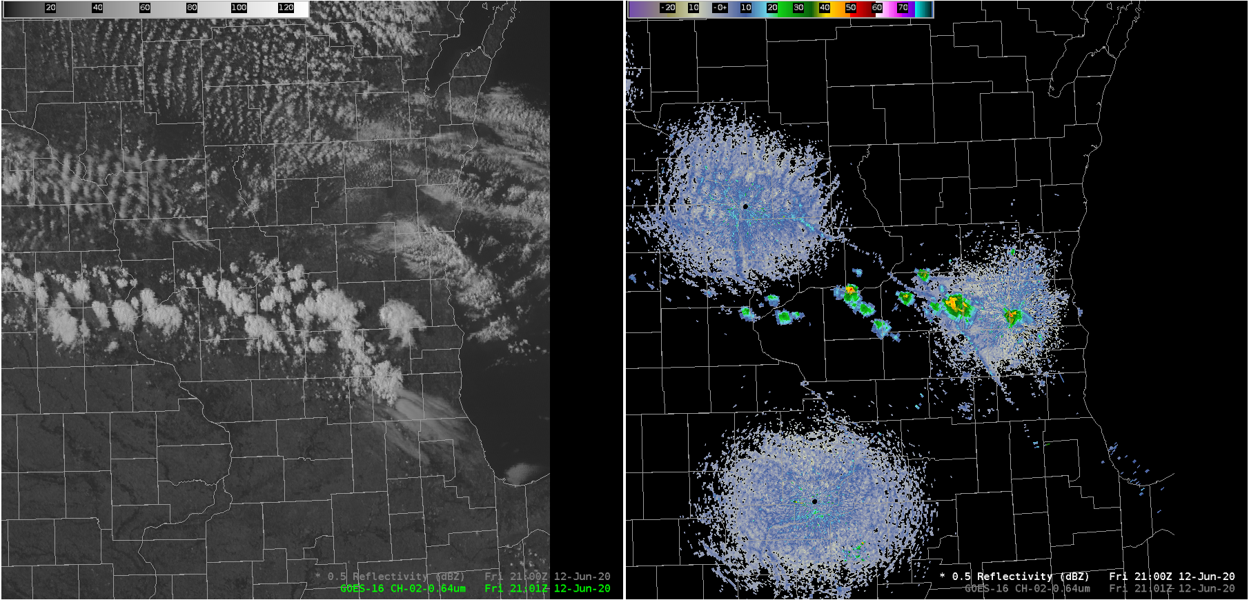
GOES-16 ABI Band 2 (0.64 ) visible imagery (left) and Midwest Composite Radar (right), 1736 – 2100 UTC on 13 June 2020 (Click to animate)
Showers developed over southern Wisconsin late in the day on 12 June 2020. What satellite products could be used to anticipate where the showers would develop? The animation of visible and radar, above, shows that the storms initiated near a boundary (mostly stationary) that separated Lake Michigan-influenced air with less stable air (based on cumuliform cloud development) to the south and west. Showers develop near the lake breeze front starting around 2000 UTC; a parallax shift is obvious between the radar and satellite (2100 UTC example) A parallax correction on the satellite imagery would shift the cloud locations towards the sub-satellite point (0, 75.2 W for GOES-East).
NUCAPS (NOAA-Unique Combined Atmospheric Processing System) soundings combine infrared and microwave information from the high spectral resolution CrIS (Cross-track Infrared Sounder) and ATMS (Advanced Technology Microwave Sounder) instruments on NOAA-20 to yield estimates of the thermodynamic structure of the atmosphere. NOAA-20 overflew the western Great Lakes shortly after 1800 UTC on 12 June, and clear skies at the time means the infrared information was complete. (In cloudy skies, NUCAPS soundings are more typically driven by ATMS data, which has coarser spectral and horizontal resolution).
The Total Totals index shown below was derived from the NUCAPS thermodynamic information. A gradient in stability exists between the most unstable air in western Wisconsin and the more stable lake-influenced air over eastern Wisconsin.
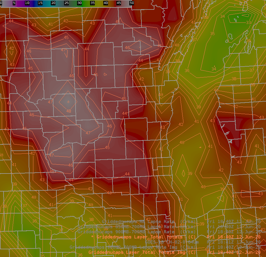
Total Totals index derived from NOAA-20 NUCAPS data, 1840 UTC on 12 June 2020 (Click to enlarge)
The low-level lapse rate, below, (from 900-700 mb), also shows a gradient in stability in the region where shower development occurred. It is not unusual for shower initiation to occur in gradients of stability (Example 1, Example 2,…), so that is a region on which to focus when waiting for convection to start.
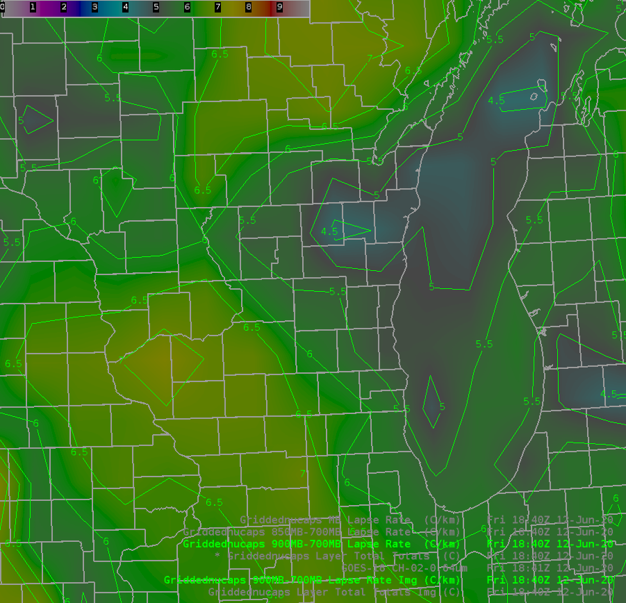
900-700 mb Lapse Rates derived from NOAA-20 NUCAPS data, 1840 UTC on 12 June 2020 (Click to enlarge)
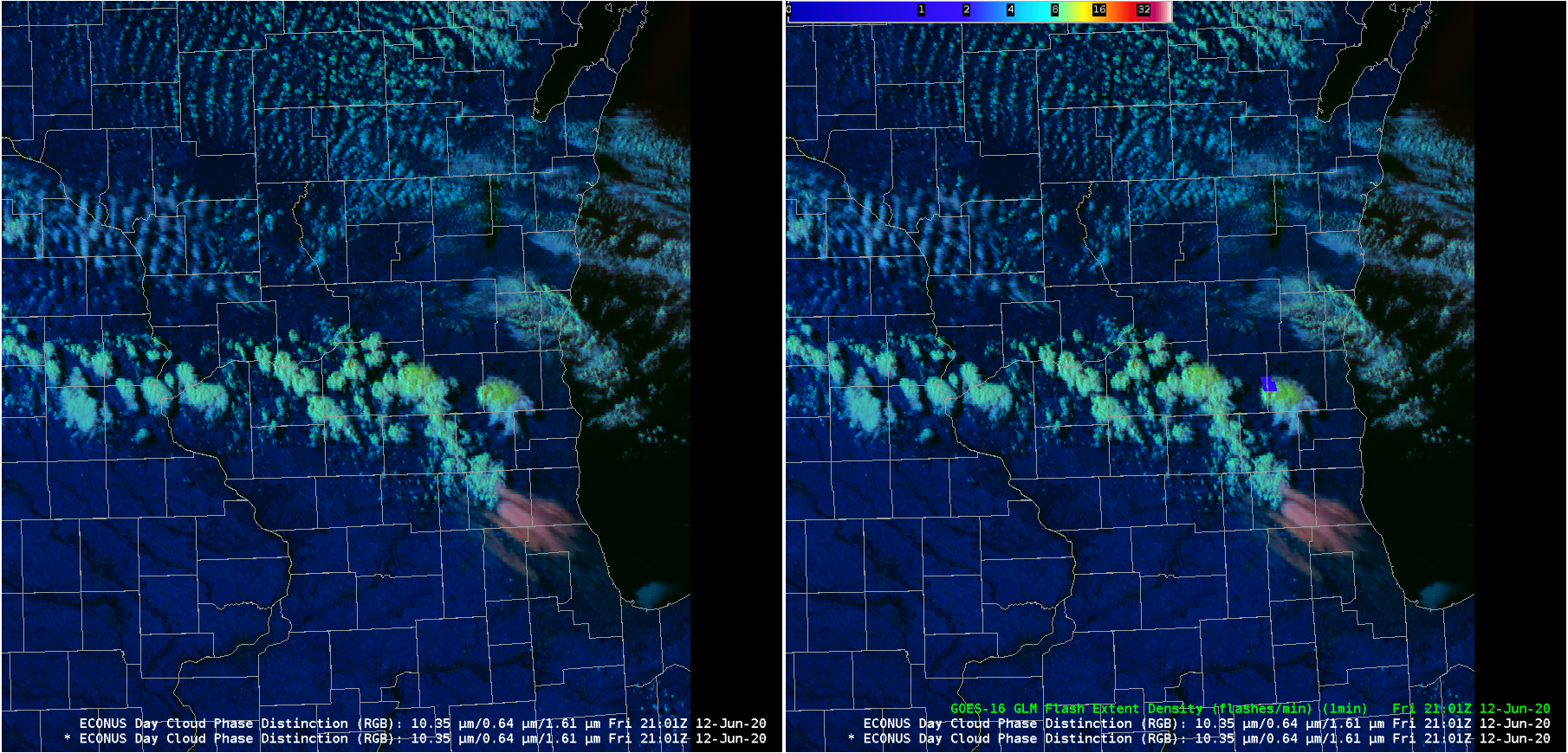
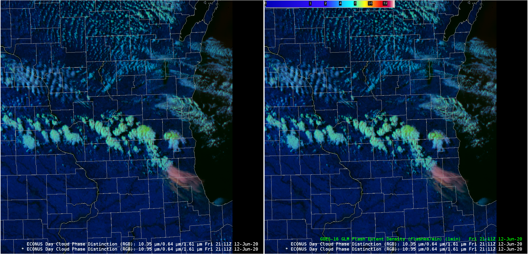
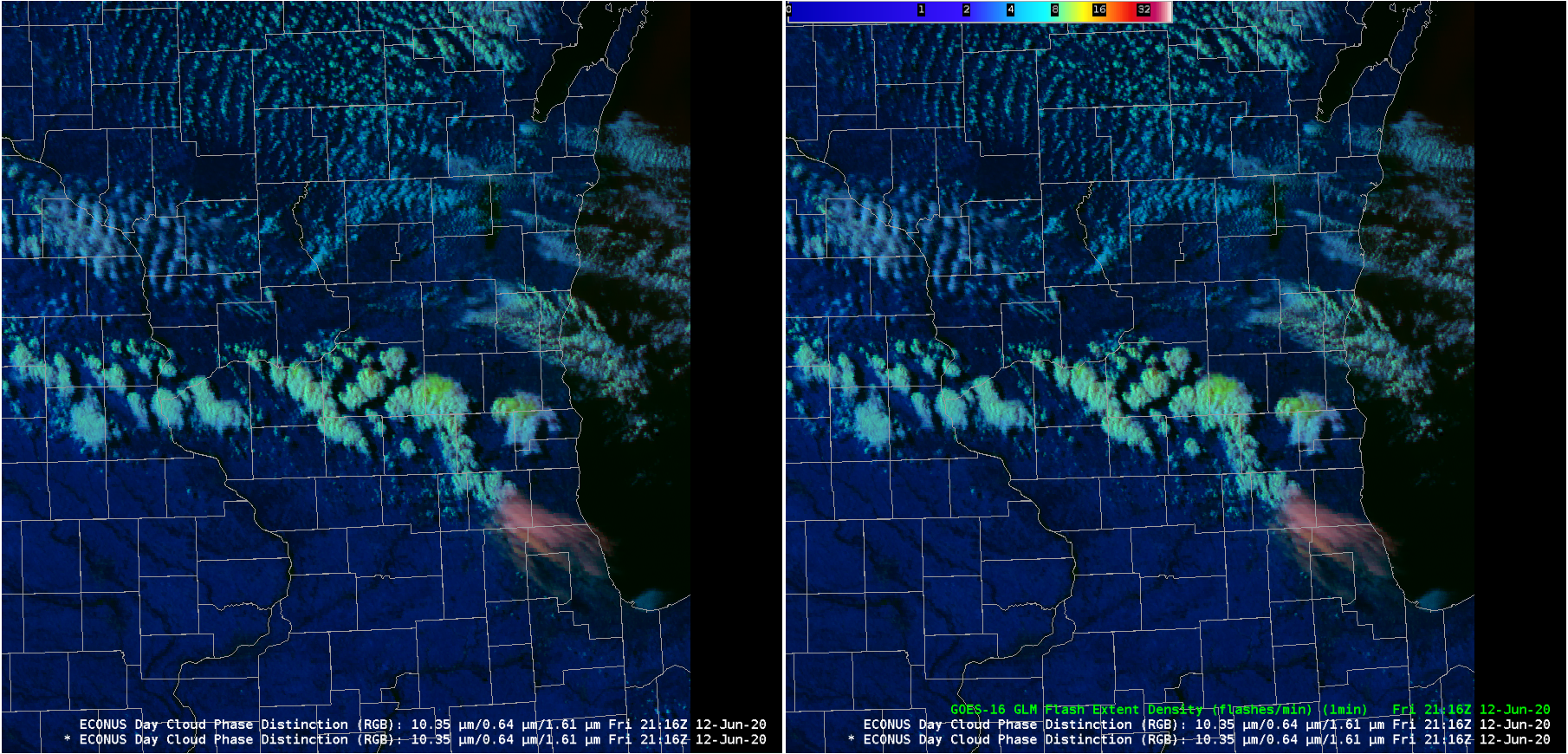
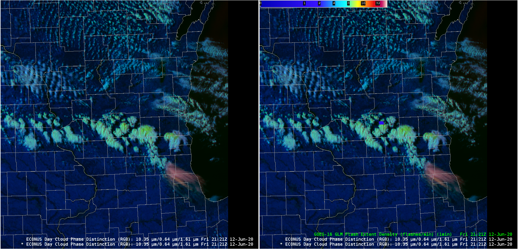
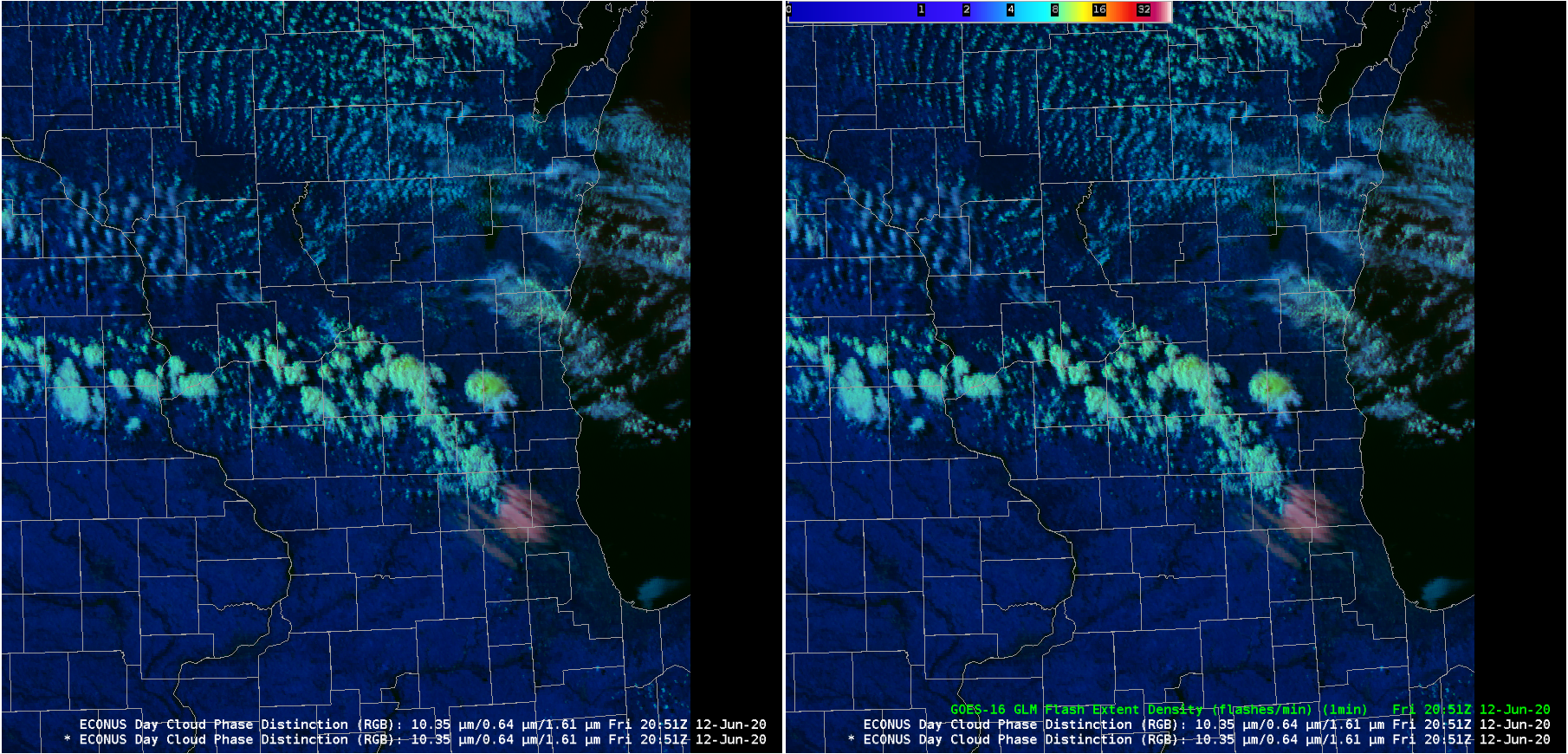
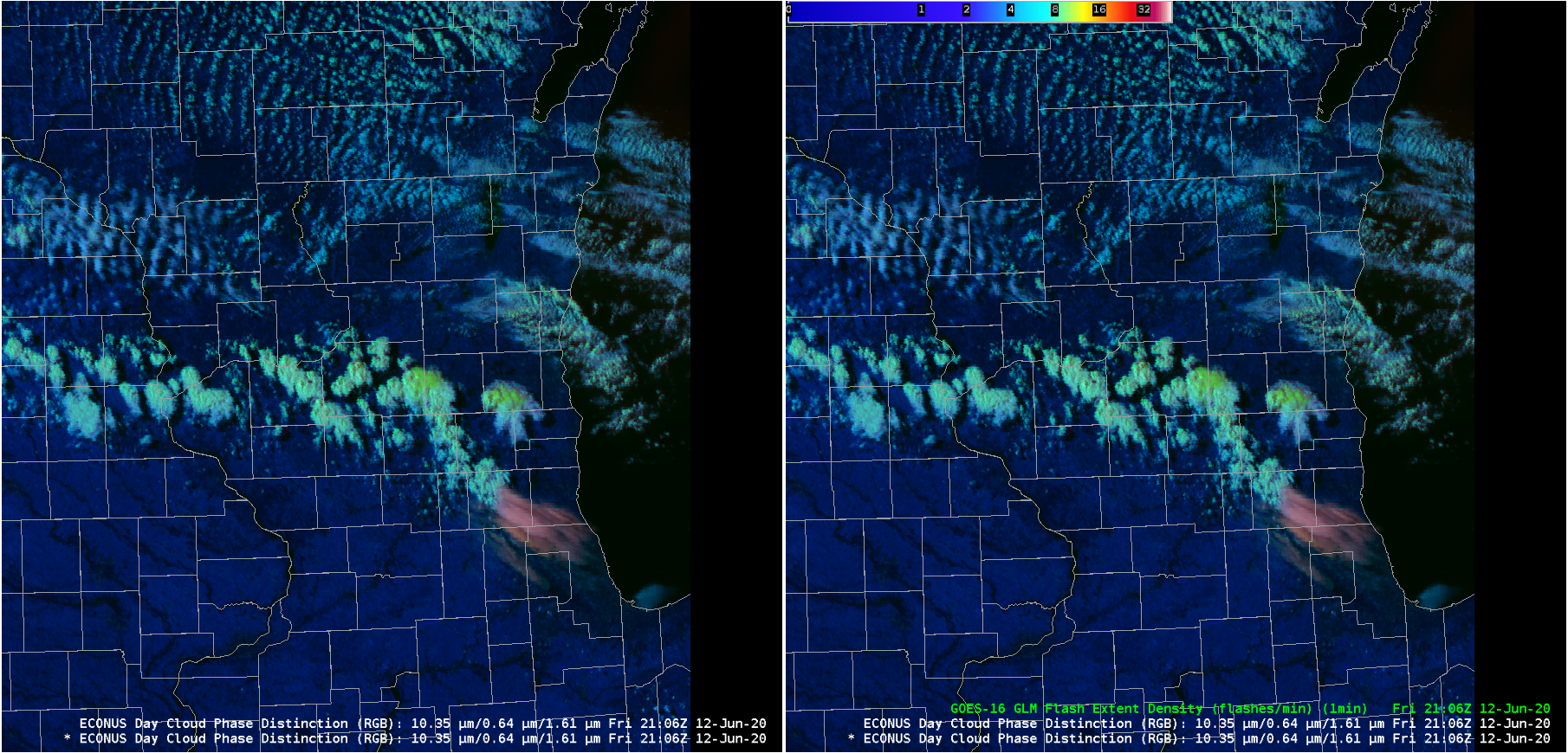
Once the shower development occurs, when will lightning occur? As noted in this blog post, the Day Cloud Phase Distinction Red-Green-Blue imagery that includes the 1.61 µm band (at which wavelength reflectance is greatly affected by the presence of ice) gives a visual clue to when glaciation occurs, and cloud-top glaciation commonly precedes lightning development. The animation below shows the Day Cloud Phase Distinction on the left, and the Day Cloud Phase Distinction overlain with Geostationary Lightning Mapper (GLM) Flash Extent Density.
There are only two detected lightning flashes in this animation — and in both cases, the Day Cloud Phase Distinction has become more orange/yellow and less green/blue before the lightning strike. This color change occurs as the 1.61 µm imagery becomes darker: ice in the cloud top increases the absorption (and reduces the reflectance) of 1.61 µm solar energy. Compare the 2111, 2116 and 2121 imagery for the lightning strike near Madison in Dane County; Similarly, compare the 2051, 2056, 2101 and 2106 imagery for the 2101 UTC lightning strike in Waukesha county). There are subtle color changes (on other days the changes are more obvious!) in the Day Cloud Phase Distinction RGB that preceded lightning events.

GOES-16 Day Cloud Phase Distinction (left), and Day Cloud Phase Distinction overlain with Geostationary Lightning Mapper (GLM) data (Click to animate)
GOES-16 Level 2 Products include Derived Stability Products (these can be found online here as well), and the mostly clear skies on 12 June meant a good signal. The Baseline Lifted Index, shown below from 1701 through 2256 UTC, shows convection developing along the eastern edge of less stable air.
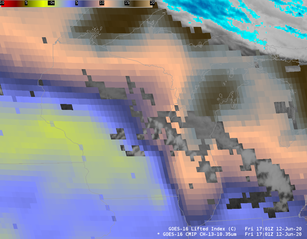
GOES-16 Derived Stability Index (Lifted Index) in clear regions, GOES-16 ABI Band 13 (10.3 µm) infrared imagery in cloud regions, 1701-2256 UTC on 12 June 2020 (Click to animate)
Is there an easily identifiable trigger that spawned these storms? Water Vapor imagery often shows impulses in clear skies. The two RGB products below combine different water vapor channels. There is a subtle increase in the amount of orange in the Differential Water Vapor before the convection starts. This increase in the red component is an increase in the brightness temperature difference between upper and lower water vapor channels, a difference that can be associated with upper-tropospheric forcing. The simple water vapor RGB (that includes the upper and lower water vapor channels, but not the difference between them) on the right shows no obvious signal.

GOES-16 Differential Water Vapor RGB (left) and SImple Water Vapor RGB (right) from 0916 to 2116 UTC on 12 June 2020 (Click to animate).
The Air Mass RGB (described here) also has the split water vapor difference as its red component. The animation below (from this site), shows a subtle change in air mass (cooler, dryer air moving southward from Canada) that could have provided an additional triggering mechanism for the convection.

GOES-16 Air Mass RGB, 1541 to 2141 UTC on 12 June 2020 (Click to enlarge)
Webcams in Madison, WI, that capture the evolution of these storms, and also show the GOES-16 imagery (derived from this site), are available at this tweet from @GOESGuy.
View only this post
Read Less
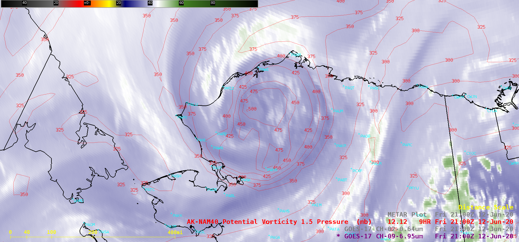
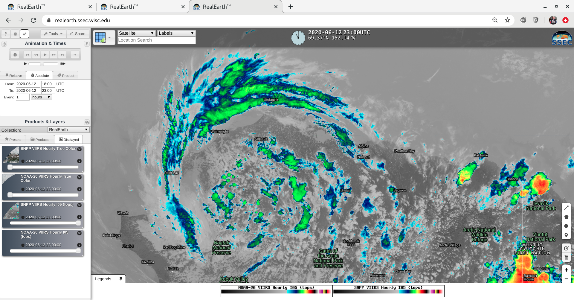
![GOES-17 Mid-level Water Vapor (6.9 µm) images, with contours of PV1.5 Pressure plotted in red [click to play animation | MP4]](https://cimss.ssec.wisc.edu/satellite-blog/images/2020/06/200612_goes17_waterVapor_pv1.5pressure_AK_anim.gif)
![GOES-17 Mid-level Water Vapor (6.9 µm) images, with contours of PV1.5 Pressure plotted in red and available NUCAPS sounding profiles denoted by green/yellow points [click to enlarge]](https://cimss.ssec.wisc.edu/satellite-blog/images/2020/06/ak_wv_nucaps-20200612_215031.png)
![NUCAPS sounding profile [click to enlarge]](https://cimss.ssec.wisc.edu/satellite-blog/images/2020/06/200612_22utc_nucaps_profile_AK.png)
![GOES-17 "Red" Visible (0.64 µm) images, with hourly surface reports plotted in red [click to play animation | MP4]](https://cimss.ssec.wisc.edu/satellite-blog/images/2020/06/200612_goes17_visible_AK_anim.gif)
![VIIRS True Color (RGB) and Infrared Window (11.45 µm) images from NOAA-20 and Suomi NPP [click to enlarge]](https://cimss.ssec.wisc.edu/satellite-blog/images/2020/06/200612_noaa20_suomiNPP_trueColorRGB_infraredWindow_AK_anim.gif)


![GOES-17 “Red” Visible (0.64 µm, top), Shortwave Infrared (3.9 µm, center) and “Clean” Infrared Window (10.35 µm, bottom) images, with hourly plots of surface reports [click to play animation | MP4]](https://cimss.ssec.wisc.edu/satellite-blog/images/2020/06/200611_goes17_visible_shortwaveInfrared_longwaveInfraredWindow_AZ_pyrocb_anim.gif)
![Plot of rawinsonde data from Tucson, Arizona [click to enlarge]](https://cimss.ssec.wisc.edu/satellite-blog/images/2020/06/200612_00UTC_KTWC_RAOB.GIF)
![Suomi NPP VIIRS True Color RGB image, with plots of VIIRS Fire Radiative Power [click to enlarge]](https://cimss.ssec.wisc.edu/satellite-blog/images/2020/06/200611_2128utc_suomiNPP_trueColorRGB_fireRadiativePower_AZ.png)
![Plot of surface observation data at Springerville, Arizona [click to enlarge]](https://cimss.ssec.wisc.edu/satellite-blog/images/2020/06/200611_KJTC_SFCMG.GIF)
