This website works best with a newer web browser such as Chrome, Firefox, Safari or Microsoft
Edge. Internet Explorer is not supported by this website.
NASA was supposed to launch its Artemis rocket to the moon this morning, at 8:33 AM EDT (12:33 UTC) from Cape Canaveral, FL. However, an engine problem caused NASA to scrub the launch for today. Even if all technical aspects of the launch were “go”, developing convection near Cape Canaveral might have posed a... Read More
NASA was supposed to launch its Artemis rocket to the moon this morning, at 8:33 AM EDT (12:33 UTC) from Cape Canaveral, FL. However, an engine problem caused NASA to scrub the launch for today. Even if all technical aspects of the launch were “go”, developing convection near Cape Canaveral might have posed a problem for the rocket launch.
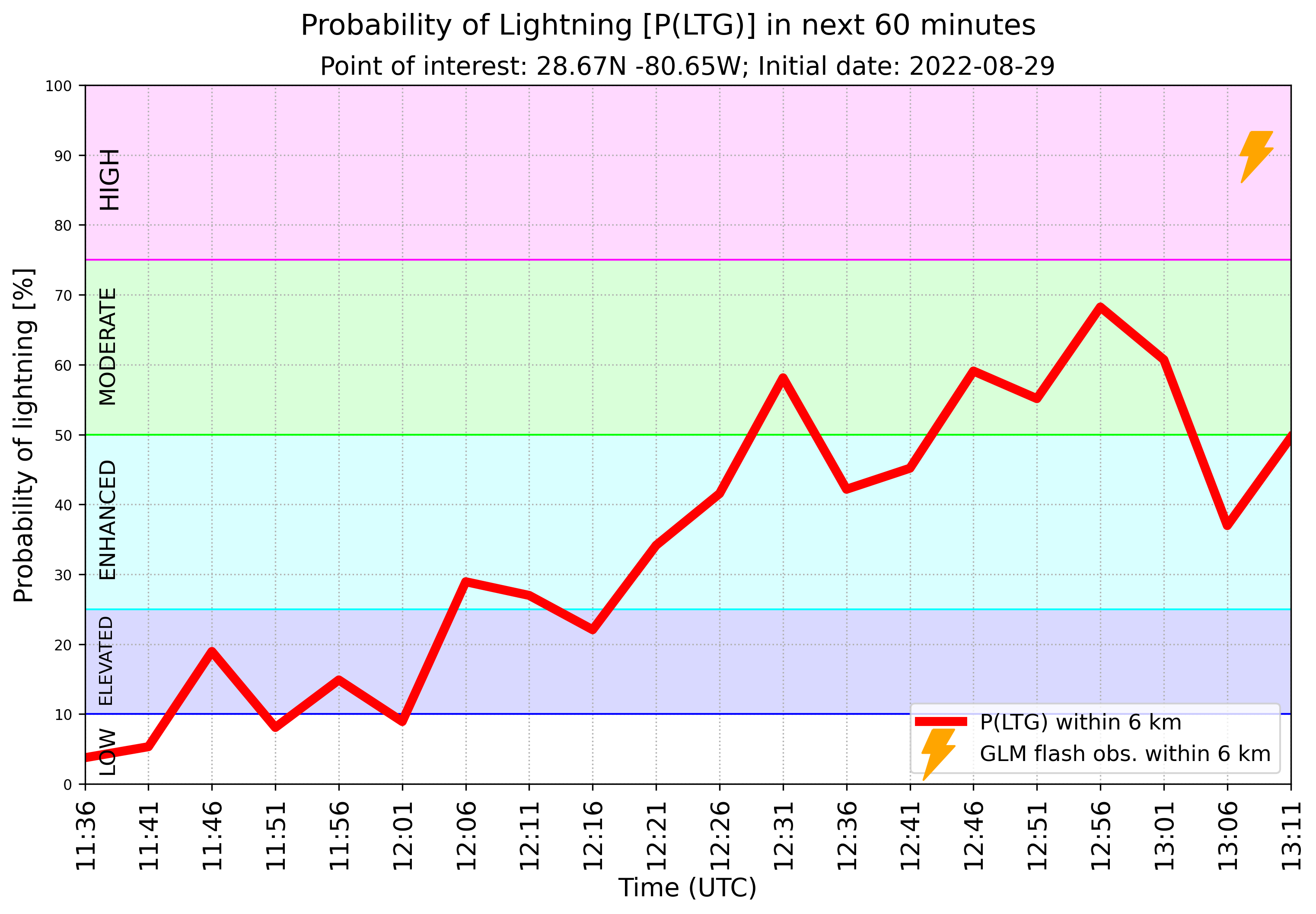
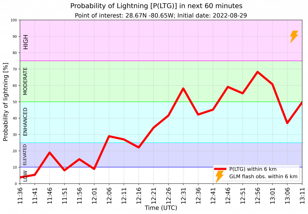
ProbSevere LightningCast, an AI model developed by CIMSS and NOAA, uses GOES-R ABI images to predict lightning in the next 60 minutes. It was predicting elevated probabilities of lightning near Kennedy Space Center prior to the start of the launch window, reaching nearly 60% by 12:31 UTC. Lightning was eventually observed by the Geostationary Lightning Mapper by 13:11 UTC.
Figure 1: GOES-East Day-Land-Cloud-Convection RGB, LightingCast contours, and GLM flash-extent density (blue boxes). The red circles represent 5-mile and 10-mile range rings around Kennedy Space Center. Figure 2: A time series of the LightningCast probability of lighting and GLM-observed lighting near Kennedy Space Center, in Cape Canaveral, FL.
Tools like LightningCast can help convert the rich information from GOES-R ABI into actionable information, helping decision-makers protect life and property. In this case, LightingCast could hypothetically be used to help protect billions of dollars of equipment, as well as the lives of NASA personnel preparing the launch pad. While this is a hypothetical case, experimental LightningCast output has been used routinely by the National Weather Service to provide guidance on lighting initiation and to inform their impacts-based decision support to key events and partners.
Seismic activity has been ongoing in August 2022 beneath the island of Ta’u to the east of American Samoa. (USGS has published a variety of information on this swarm of Earthquakes: link 1; link 2; link 3); See also these two recorded Facebook Live presentations from the NWS WSO office in Pago Pago:... Read More
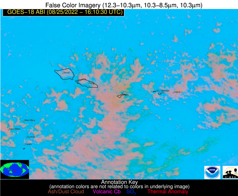
False Color imagery over the American Samoa sector, 1610 UTC on 25 August 2022 (Click to enlarge)
Seismic activity has been ongoing in August 2022 beneath the island of Ta’u to the east of American Samoa. (USGS has published a variety of information on this swarm of Earthquakes: link 1; link 2; link 3); See also these two recorded Facebook Live presentations from the NWS WSO office in Pago Pago: (August 22nd and August 17th). Volcano updates fro Ta’u can also be viewed here.
The Volcanic Ash Advisory Center (VAAC) that has responsibility for this region of the south Pacific is Wellington NZ. Click here for a pdf that shows all VAAC boundaries.
Should an eruption occur (NOTE: An eruption is not expected in the near term!), what kind of satellite information will be useful? The Volcanic Cloud Monitoring website (link) from CIMSS includes imagery over various sectors on Earth, sorted by VAAC. For American Samoa, and adjacent regions, Choose ‘Satellite Imagery’ and under the ‘Sector’ menu, and then choose, under the Wellington VAAC subsection, ‘American Samoa (750 m)’ Both GOES-17 / GOES-18 and Himawari view the region, but GOES-17/GOES-18 sub-satellite points are closer to American Samoa and will provide better resolution views. (NOAA-20 and Suomi-NPP as polar orbiters will provide the highest spatial resolution data, but have poor temporal resolution). You can choose various image types at the website: quantitative estimates of Ash Loading, Ash Height, Ash Loading, Ash Reflectivity, Single-channel Brightness Temperatures (or Reflectivity), and various Red/Green/Blue composites. Note that this website has an extensive explanatory section (under the ‘Tutorials’ tab) to help you understand what you’re seeing in the imagery. The GOES-18 false-color image red/green/blue image, above, is the from the website. An eruption is not occurring, nor detected, in the image.
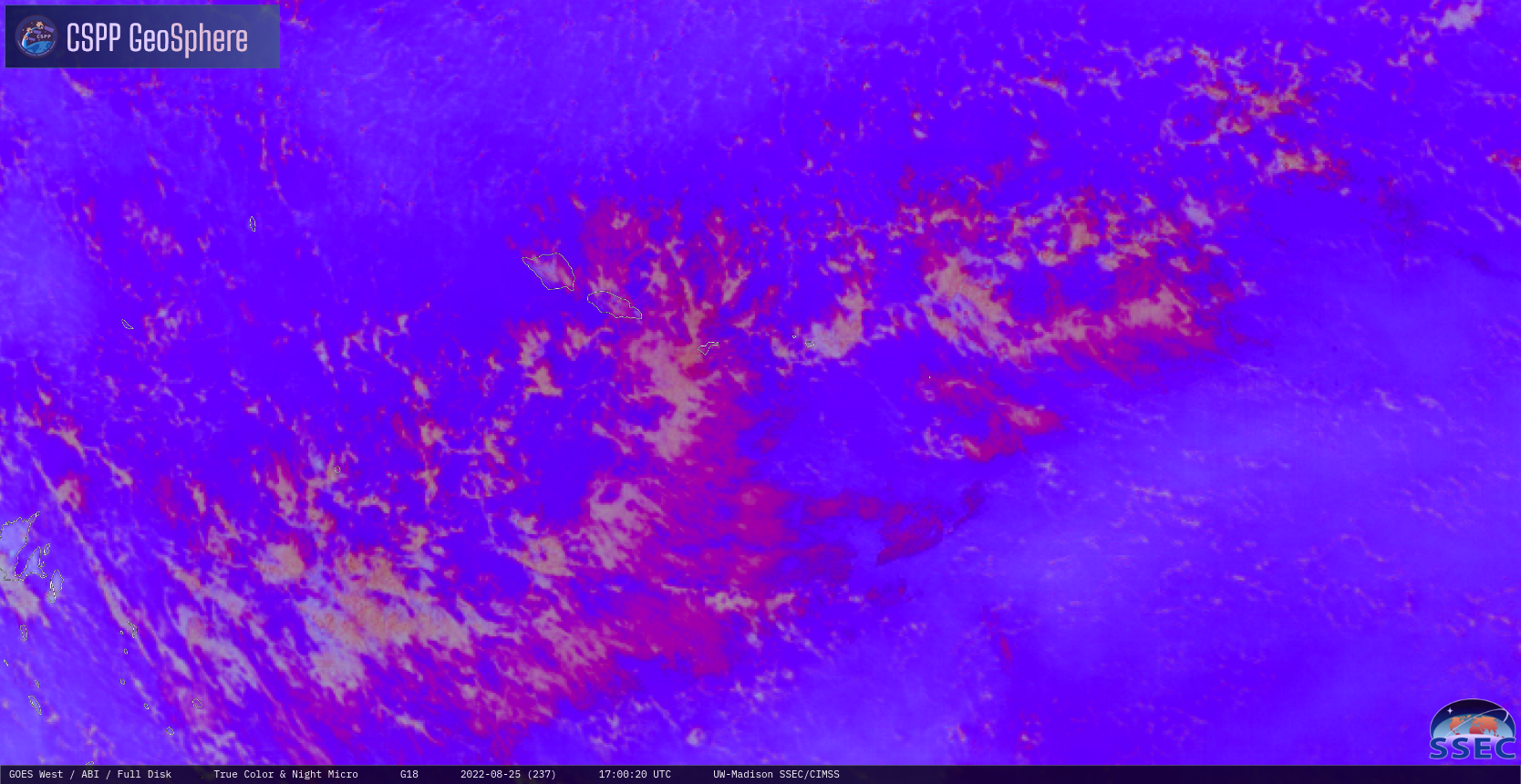
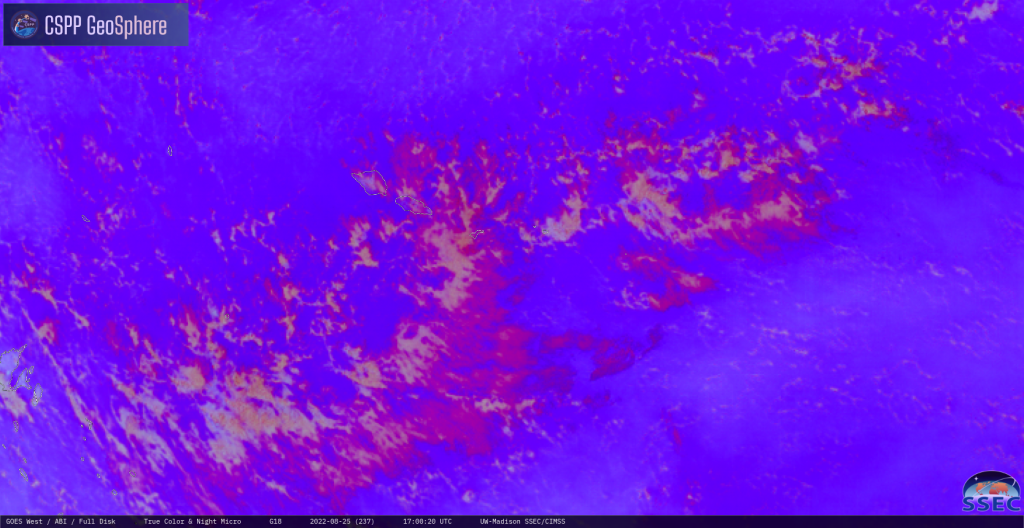
Various websites also allow views of Satellite Imagery over the region. For example, the CSPP Geosphere site includes True-Color imagery (day) and Night time Microphysics (night) by default, but also allows a user to view single channels. (Direct link, see an example below) There is also a NOAA/NESDIS site that includes some RGBs and each of the individual bands; the CIRA Slider also includes imagery over the south Pacific.
Night Microphysics RGB near American Samoa, 1700 UTC on 25 August 2022 (Click to enlarge)
Wind direction will be important if an eruption occurs (this is at present unlikely!!) to know as that will control the dispersion of any gases. The windy.com website will provide this with this link.
This blog entry is meant to be a resource should an eruption occur. (Note: that is not expected!) For more information, please refer to the USGS website, and the American Samoa Facebook page.
GOES-7 Infrared (11.35 um) images (above) showed Hurricane Andrew making landfall along the southeast coast of Florida — as a Category 5 storm — around 0831 UTC on 24 August 1992. At that time, the coldest cloud-top infrared brightness temperatures of the eyewall region were around -75ºC. These images were created... Read More
GOES-7 Infrared (11.35 um) images [click to play animated GIF | MP4]
GOES-7 Infrared (11.35 um) images (above) showed Hurricane Andrew making landfall along the southeast coast of Florida — as a Category 5 storm — around 0831 UTC on 24 August 1992. At that time, the coldest cloud-top infrared brightness temperatures of the eyewall region were around -75ºC. These images were created using archived data from SSEC Satellite Data Services.
More information on Andrew can be found in this video produced by NWS Miami for the 25th anniversary of the storm.
Access to SSEC’s Data Center allows for some serious “data crunching” with the full record of GOES-17 ABI data. In Figure 1 below, GOES-17 Band 13 Full Disk brightness temperatures have been averaged for each month in 2021. These fields of averaged brightness temperature are useful for assisting forecasters in... Read More
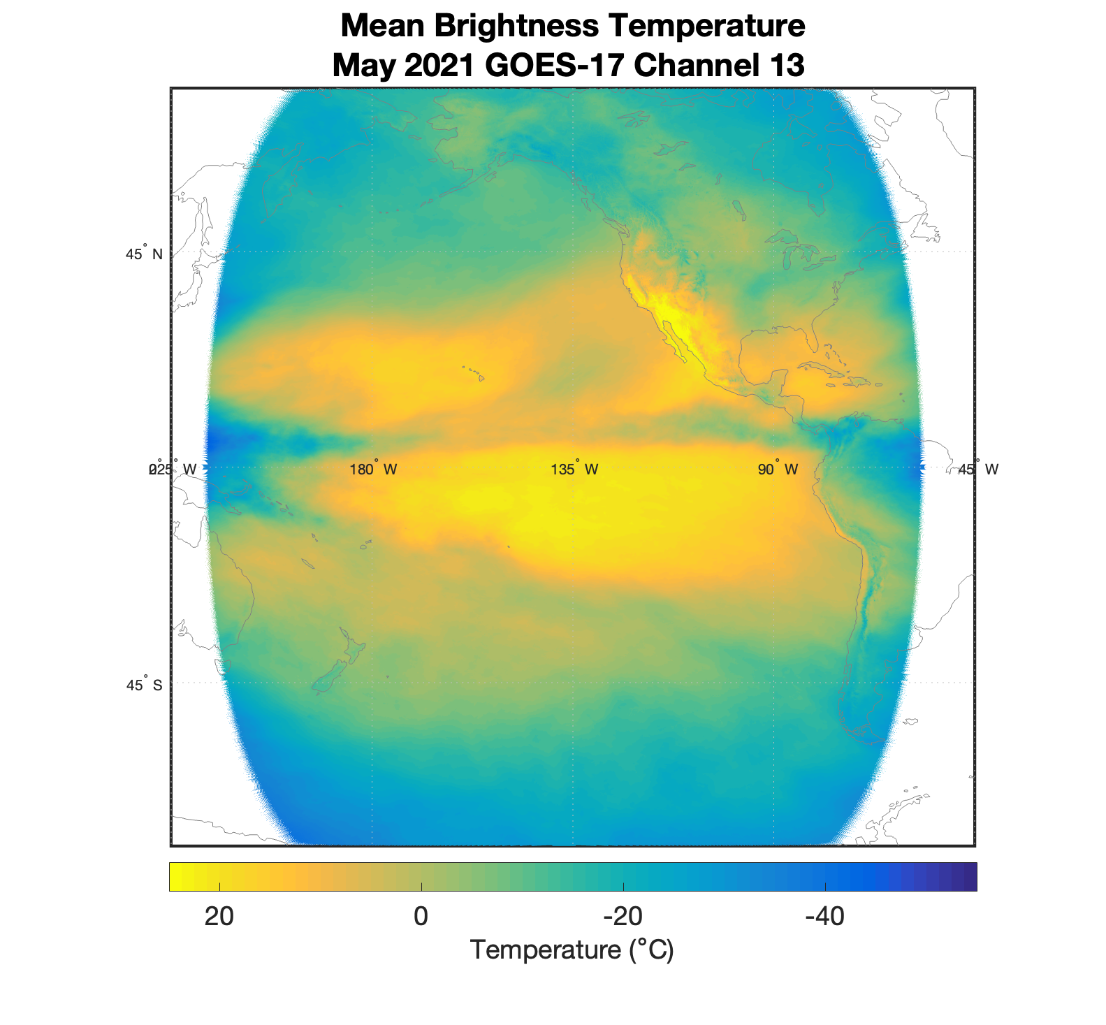
Access to SSEC’s Data Center allows for some serious “data crunching” with the full record of GOES-17 ABI data. In Figure 1 below, GOES-17 Band 13 Full Disk brightness temperatures have been averaged for each month in 2021. These fields of averaged brightness temperature are useful for assisting forecasters in knowing what can be expected from satellite retrievals on monthly timescales, especially in remote Pacific regions where forecasters are heavily reliant on satellite data.
Figure 1. An animation of monthly mean GOES-17 Band 13 Full Disk brightness temperatures for 2021. [Click to open in new tab.]
2021 was a typical La Nina year, which is associated with dry weather in the Southwest United States. A strong surface heat signal can be seen in that region from April – September.
May – October experiences cooler temperatures in the East Pacific near Mexico and Central America. This may be associated with the 2021 Pacific Hurricane season.
Figure 2 is the same animation for tropical latitudes only. In all months, the ITCZ band is visible. It can be recognized as a band of cooler brightness temperatures (green-teal color) that sits slightly north of the equator. If you look closely, the ITCZ seems to undergo a slight northward migration as the year progresses. This northward shift is more noticeable in the transitions from April to May and from September to October.
Figure 2. An animation of tropical monthly mean GOES-17 Band 13 brightness temperatures for 2021. [Click to open in new tab.]

