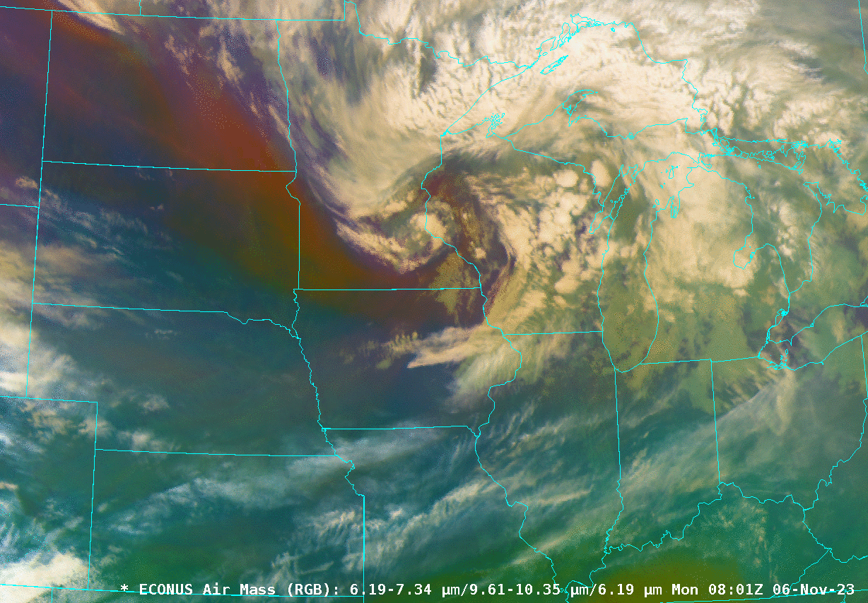
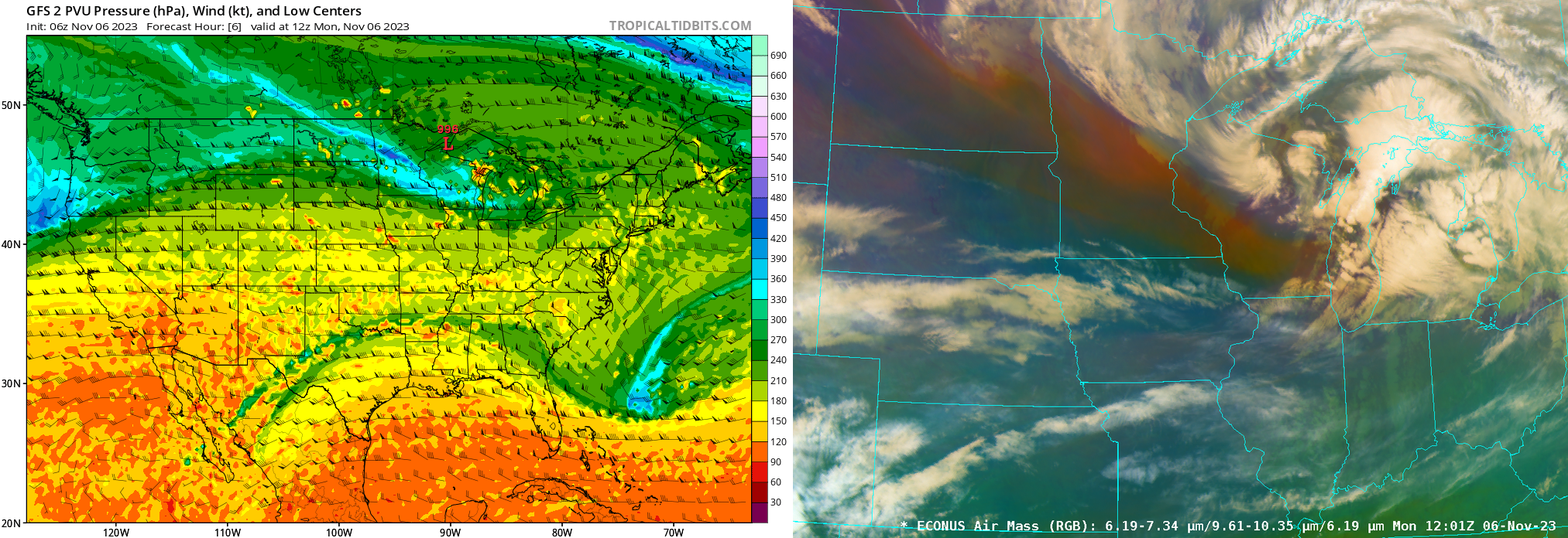
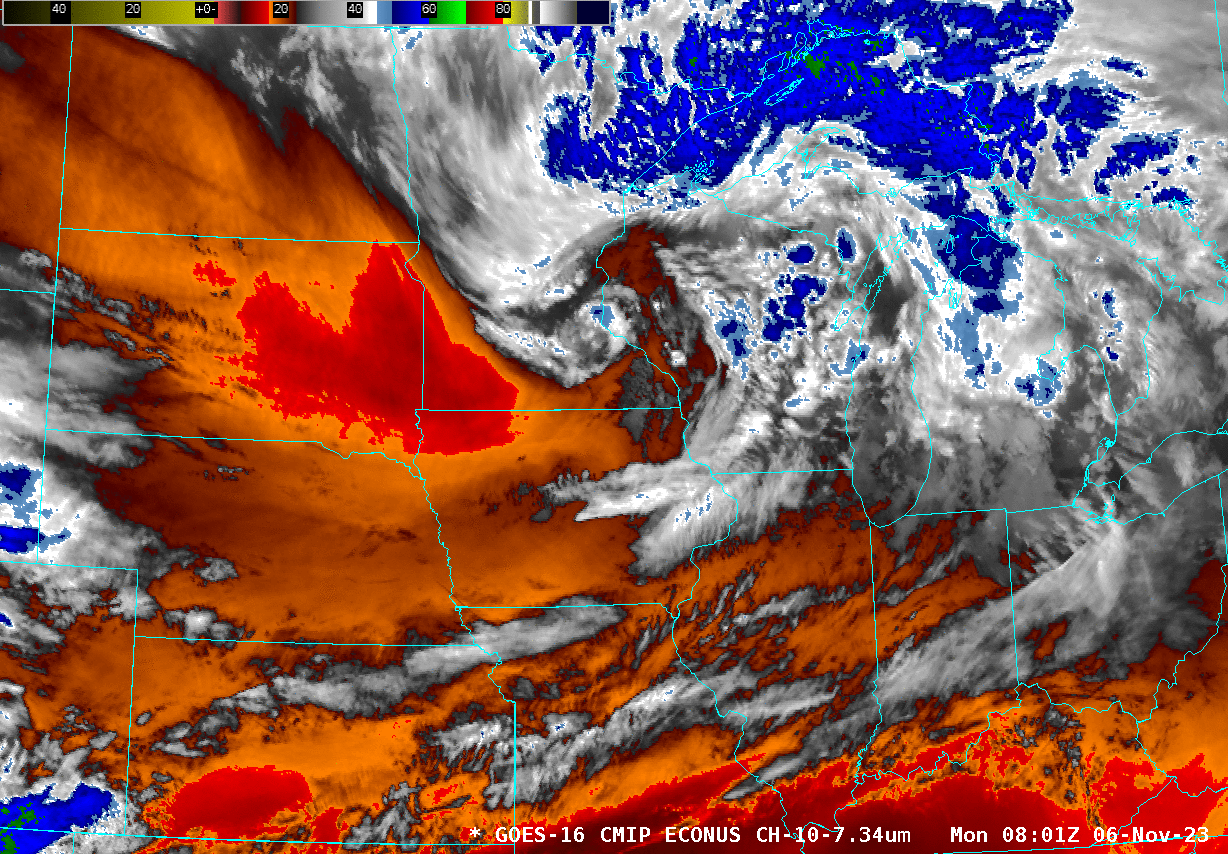
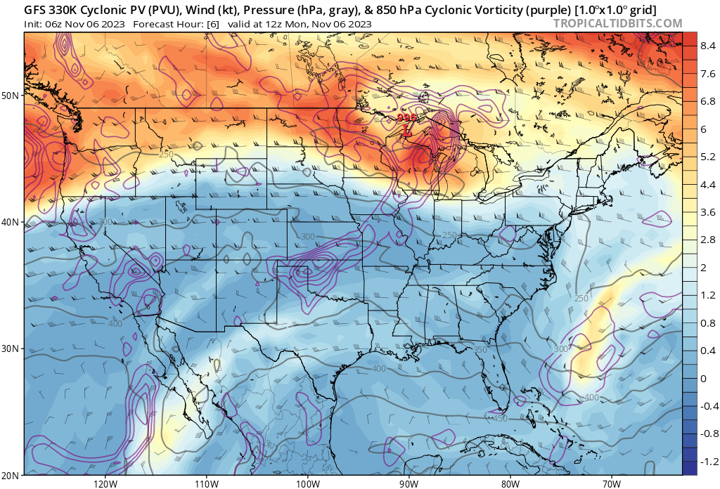
Storm Reports for the first two weeks of November 2023 show that the all but one of the reports have occurred over lower Michigan, where large hail (1 to 1.5 inches in diameter) occurred shortly after sunrise on 6 November in Newaygo County (1423 UTC), Montcalm County (1440, 1443 UTC) and Kent County (1448 UTC). What satellite imagery could be used to monitor this out-of-season development? The airmass RGB animation, above, from 0801 – 1501 UTC, shows the orangish shading typical of an airmass with high potential vorticity impinging on western Lower Michigan. Is that orange region really a region where Potential Vorticity is elevated? The image below compares the 1200 UTC (6-h GFS forecast) of pressure on the 2 PVU (taken from this source) to the 1201 UTC Airmass RGB. Strong convection develops over Lake Michigan after 1200 UTC and moves into southwestern lower Michigan where the severe weather occurred around 1400 and 1500 UTC.
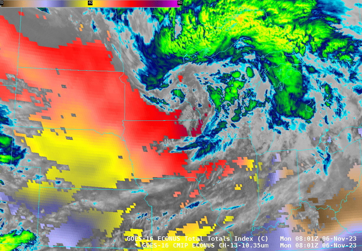
GOES-R provides Derived Stability Indices as one of its Level 2 Products. The clear-sky stability products include the Total Totals Index and the animation below shows the values along with the GOES-16 Clean Window infrared imagery. Values in excess of 45 occasionally appear in clear sky pixels over western lower Michigan as the stronger convection develops. Values are even larger to the west/southwest over Wisconsin where dynamic forcing is presumably less strong (given that convection did not develop there; here is a 6-h forecast of pressure on the 330 K surface along with cyclonic vorticity at 850 mb; note the strongest dynamics at 12 UTC are over northeast WI).
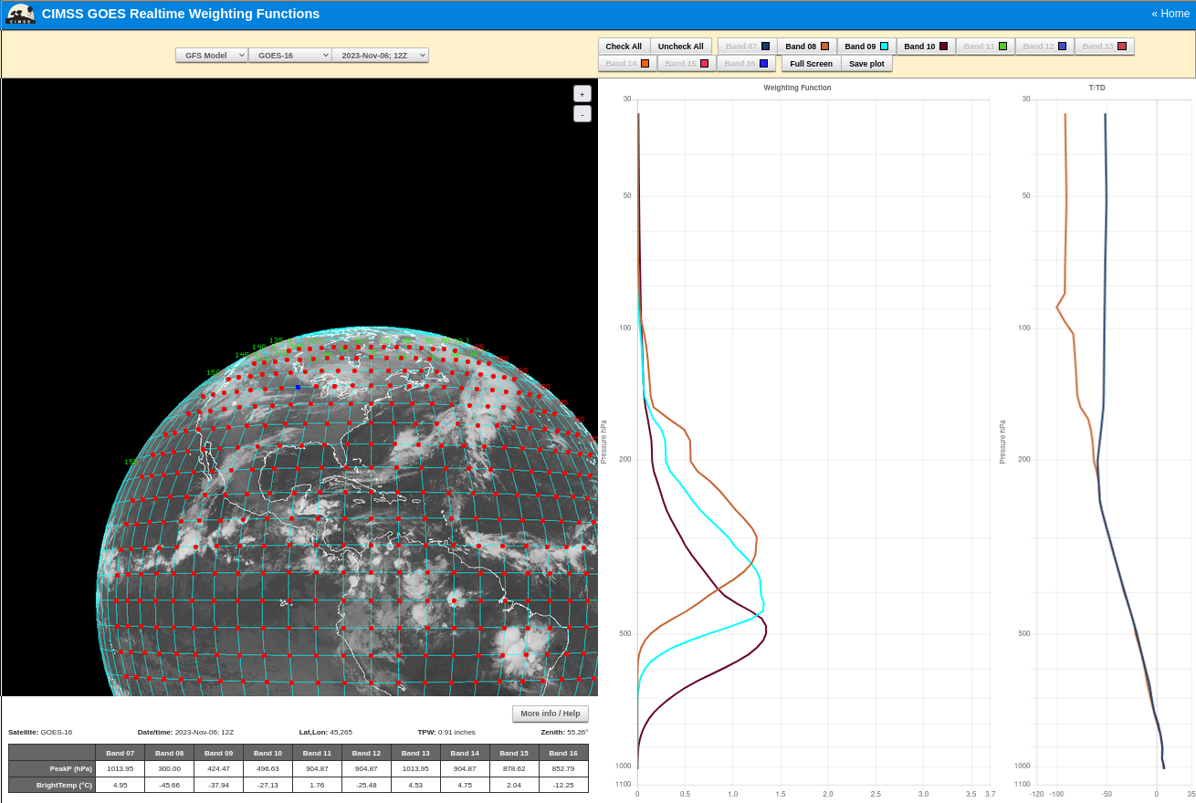
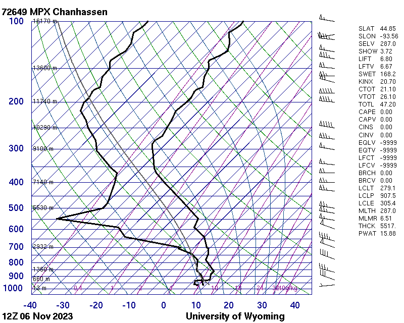
GOES-16 low-level water vapor imagery, below, shows the characteristic red signature sometimes associated with Elevated Mixed Layers (EMLs, features that are conducive to convection) moving towards lower Michigan. The weighting function from 45 N, 95W computed from 1200 UTC 6 November 2023 GFS data (here, taken from this source), shows a peak contribution from near 500 mb. The 1200 UTC Chanhassen Minnesota soundings (here, from this source), shows near dry-adiabatic conditions at 500 mb, i.e, a possible EML; if convection reaches that level, one might expect vigorous ascent.
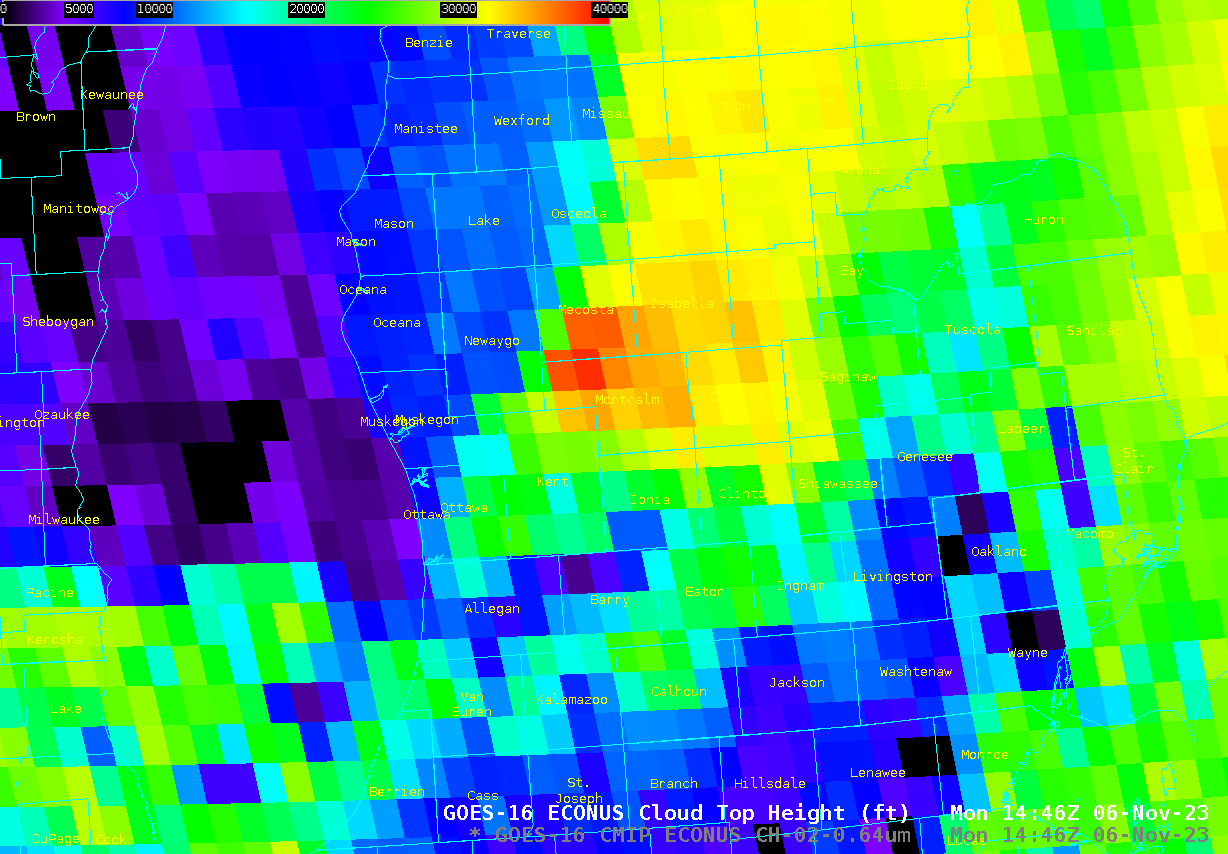
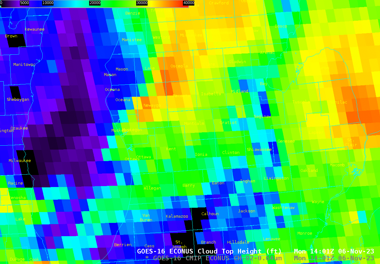
GOES-16 Visible imagery, below, colored by the L2 cloud height product, shows both the convective texture of the clouds over Newaygo, Montcalm and Kent counties, and the relatively high heights of those clouds.
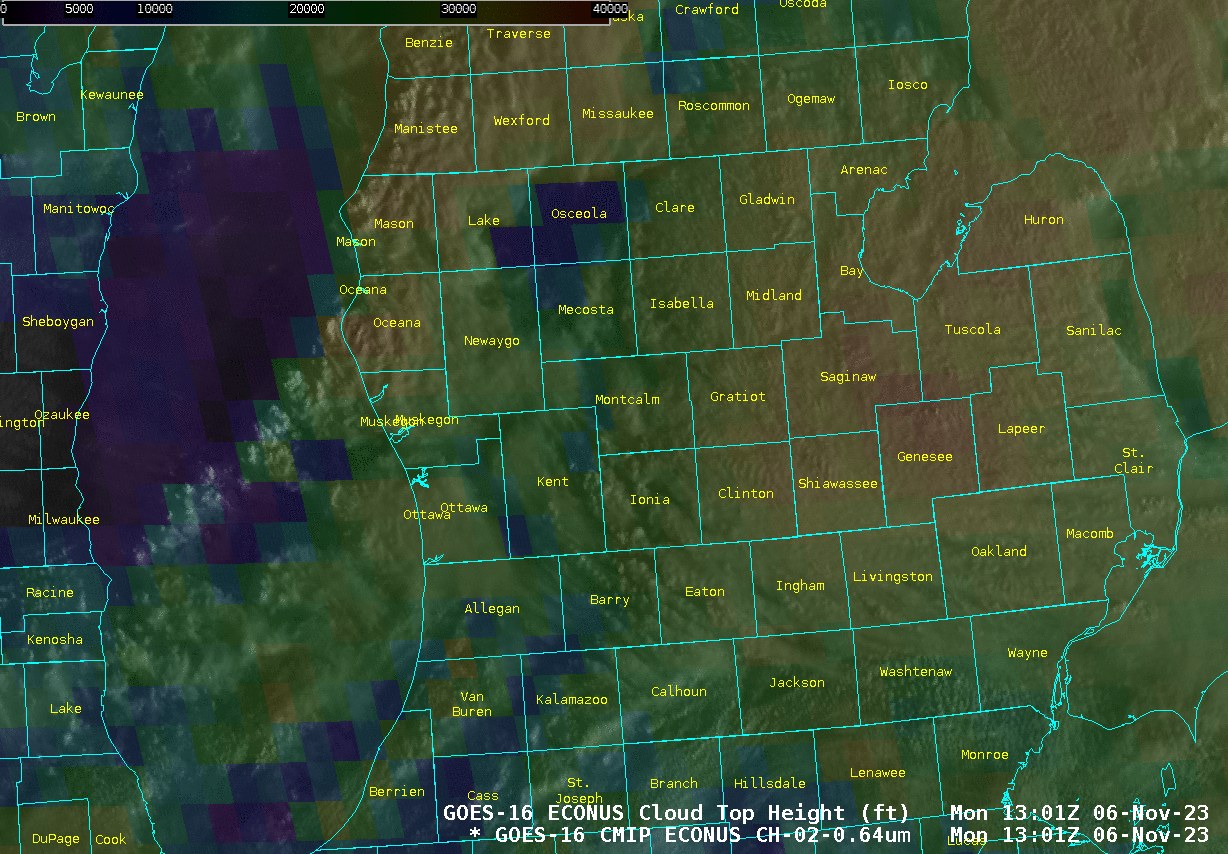
GOES-16 Cloud Top Heights, below, from 1401-1456 UTC, show the highest clouds tracking across southern Newaygo county and northern Kent and Montcalm counties from 1426 – 1451 UTC.
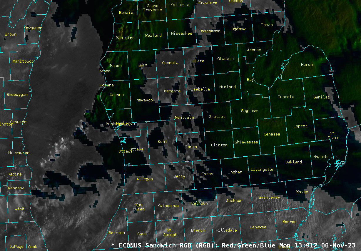
The visible imagery colored with the cloud-top height mimics what happens with the Sandwich RGB, shown below. For this RGBs, the default scaling from 0-255 was changed to 0-150 for this early morning/low light event. The cold cloud tops of the strongest convection are apparent, tracking in the same region of Newaygo/Montcalm/Kent counties between 1400 and 1500 UTC, when the severe weather was occurring.
A GOES-16 Mesoscale Domain Sector provided 1-minute imagery over the area — Visible and Infrared images that included time-matched (+/- 3 minutes) plots of SPC Storm Reports (in Newaygo/Montcalm/Kent counties) are shown below. In the vicinity of the hail reports, overshooting tops were evident in the Visible images and cloud-top 10.3 µm infrared brightness temperatures were as cold as -60ºC (darker red enhancement).
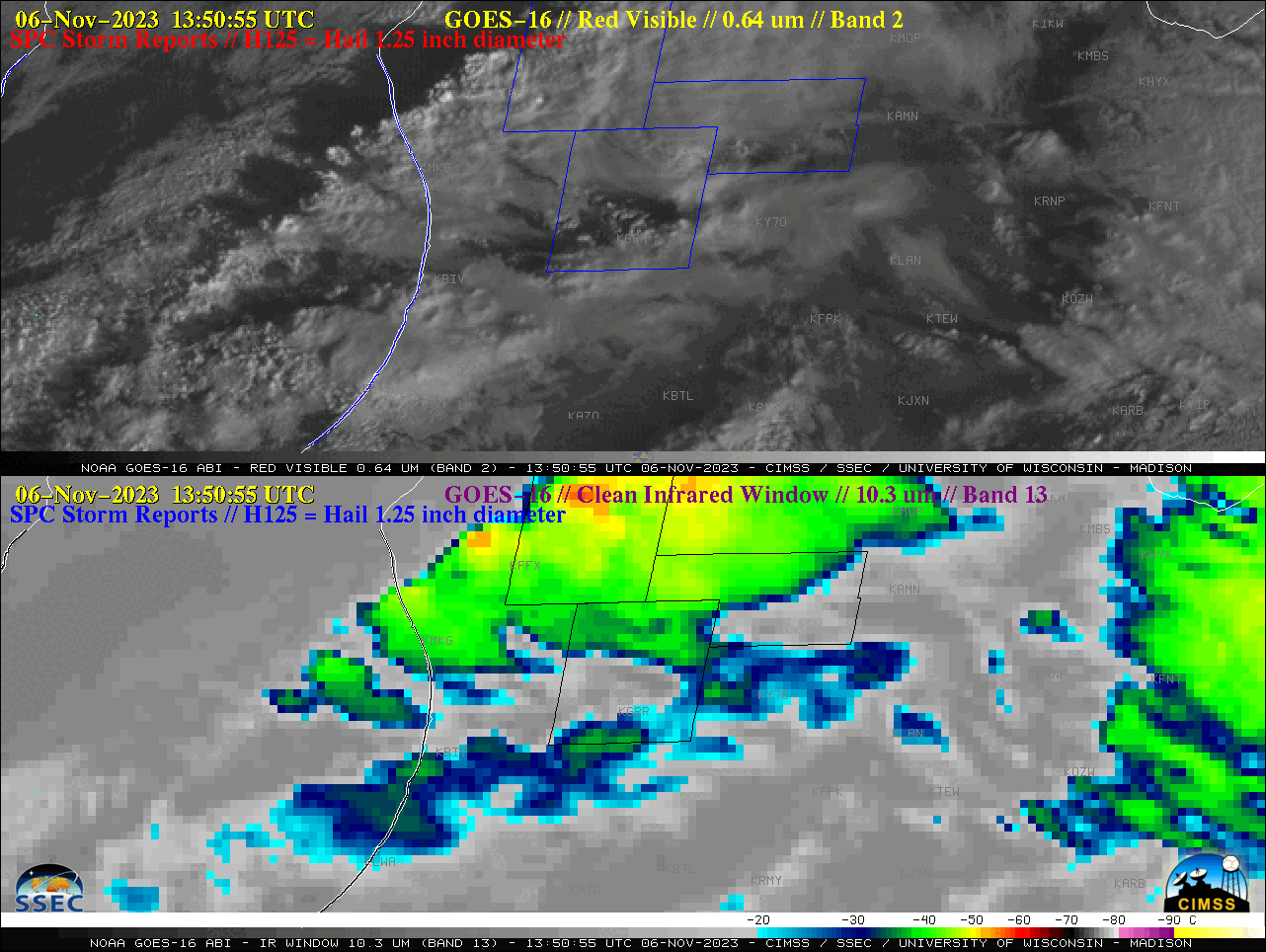
1-minute GOES-16 “Red” Visible (0.64 µm, top) and “Clean” Infrared Window (10.3 µm, bottom) images, with time-matched plots of SPC Storm Reports in Newaygo/Montcalm/Kent counties (courtesy Scott Bachmeier, CIMSS) [click to play animated GIF | MP4]
Thanks to TJ Turnage, Science and Operations Officer (SOO) at the Grand Rapids MI forecast office, for alerting us to this event.
View only this post Read Less


