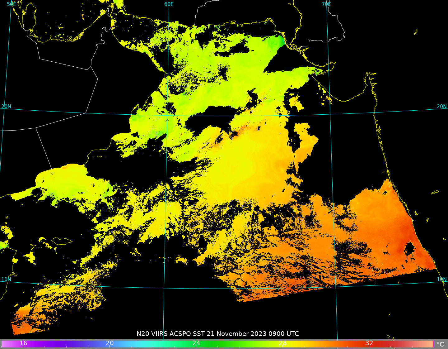

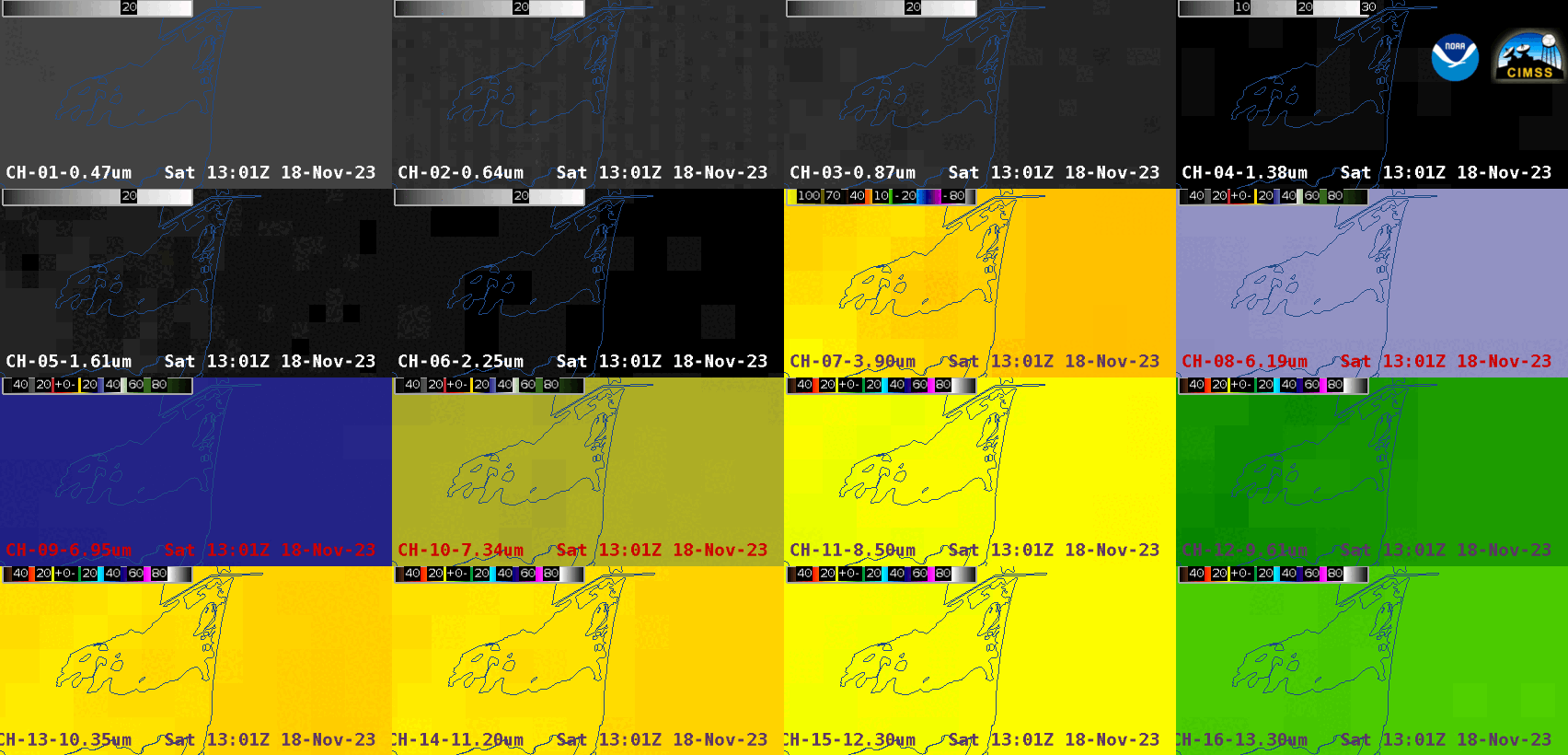
The Community Satellite Processing Package (CSPP) allows a user to manipulate VIIRS data to create high-quality, full-resolution imagery (see, for example, this I05 example, and this Day Night Band example, and this I01 example). In addition to single-band images, imagery for products such as Advanced Clear Sky Processor for Ocean (ACSPO) sea-surface temperatures (SSTs) can also be created, as shown above. Polar2grid software is being used for all examples in this blogpost. It is a Linux-based software package that is available for free download here.
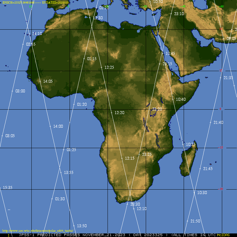
ACSPO SST data derived from VIIRS data are available online here (for Suomi-NPP) and here (for NOAA-20). Data files appear about 1-3 days after observation (a user with a Direct Broadcast antenna, of course, can process data for the needed SST files in near-real time); the two files I downloaded (from this source directly; it is also accessible via NOAA CLASS — see the note at the NOAA CLASS website and click through to the NOAA-20 site) include 10 minutes of VIIRS ACSPO observations from NOAA-20: from 09:00:00 to 09:09:59 and from 21:30:00 to 21:39:59) on 21 November 2023. This map (from this source) shows that the observations are over the Arabian Sea. The downloaded files have a file naming structure shown below
20231121090000-OSPO-L2P_GHRSST-SSTsubskin-VIIRS_N20-ACSPO_V2.80-v02.0-fv01.0.nc
20231121213000-OSPO-L2P_GHRSST-SSTsubskin-VIIRS_N20-ACSPO_V2.80-v02.0-fv01.0.nc
Several steps are needed before the imagery shown above is created. First, I defined a grid using Polar2Grid software (that is, p2g_grid_helper.sh) onto which the data are placed, because the orbit paths at 0900 and 2130 do not sample the same domain. That command is shown below.
$POLAR2GRID_HOME/bin/p2g_grid_helper.sh Arabian 63.5 14.6 2000 -2000 1440 1120 > $POLAR2GRID_HOME/Arabian.yamlBecause I know beforehand the range of sea-surface temperatures that are likely in November in the Arabian Sea, I can instruct (via a yaml file that I named “my_sst_rescale.yaml“) Polar2Grid to scale the computed SSTs appropriately. The contents of the file, that I placed in $POLAR2GRID_HOME/bin, are shown below. I’m constraining the temperatures to be between 15oC and 35oC.
enhancements:
  oman_sst:
    standard_name: sea_surface_subskin_temperature
    operations:
      - name: linear_stretch
        method: !!python/name:satpy.enhancements.stretch
        kwargs: {stretch: 'crude', min_stretch: 288.16, max_stretch: 308.16}
The polar2grid commands to (1) create the .tif file (run from the $POLAR2GRID_HOME/bin directory) is below, and (2) to apply a colormap to the two tif files (one at 0900, one at 2130) are shown below; the wildcard ‘20231121???0’ in the file name resolves the files containing both 0900 and 2130 UTC data. The two filenames created are shown beneath the polar2grid command. The add_colormap.sh command overwrites the .tif file, adding colormap information from the file p2g_sst_palette.txt, a colormap that is supplied with the polar2grid installation; a user could, of course, alter the colormap to something of their own choosing.
$POLAR2GRID_HOME/bin/polar2grid.sh -r acspo -w geotiff -p sst -g Arabian --grid-configs $POLAR2GRID_HOME/Arabian.yaml --fill-value 0 --extra-config-path my_sst_rescale.yaml -f /path/to/J01Data/20231121???0*SST*N20*

noaa20_viirs_sst_20231121_090000_Arabian.tif
noaa20_viirs_sst_20231121_213000_Arabian.tif

$POLAR2GRID_HOME/bin/add_colormap.sh $POLAR2GRID_HOME/colormaps/p2g_sst_palette.txt noaa20_viirs_sst_20231121_???000_Arabian.tif
The imagery above includes coastlines, borders, and a labeled colorbar. Those are all added with the following commands, one for each time.
$POLAR2GRID_HOME/bin/add_coastlines.sh --add-coastlines --add-borders --add-grid --grid-D 10 10 --grid-d 10 10 --grid-text-size 16 --add-colorbar --colorbar-text-color "white" --colorbar-text-size 20 --colorbar-title "N20 VIIRS ACSPO SST 21 November 2023 0900 UTC" --colorbar-height 32 --colorbar-tick-marks 4 --colorbar-min 15.0 --colorbar-max 35.0 --colorbar-units "°C" noaa20_viirs_sst_20231121_090000_Arabian.tif
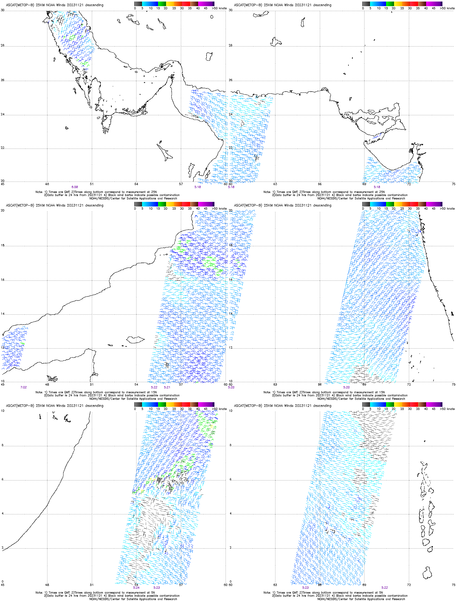
$POLAR2GRID_HOME/bin/add_coastlines.sh --add-coastlines --add-borders --add-grid --grid-D 10 10 --grid-d 10 10 --grid-text-size 16 --add-colorbar --colorbar-text-color "white" --colorbar-text-size 20 --colorbar-title "N20 VIIRS ACSPO SST 21 November 2023 2130 UTC" --colorbar-height 32 --colorbar-tick-marks 4 --colorbar-min 15.0 --colorbar-max 35.0 --colorbar-units "°C" noaa20_viirs_sst_20231121_213000_Arabian.tifNote the warmer temperatures during the daytime (i.e., at 0900 UTC). The difference between day and night will be especially pronounced in regions of reduced vertical mixing in the ocean (that is, light winds), and MetopB ASCAT winds on the 21st (below, from here) do show light winds over much of the Arabian Sea early on the 21st.
View only this post Read Less
